VLOOKUP from another or across sheets is not so complicated in Google Sheets. It depends on how you refer to several ranges in one go.
Learning how to do it is very important if you want to find information from multiple sheets in a workbook.
Even if we have XLOOKUP, VLOOKUP is the ultimate solution to get matrix Lookup outputs.
In XLOOKUP, if we specify multiple search keys, the result range won’t return results from more than one column.
Syntax: XLOOKUP(search_key, lookup_range, result_range, [missing_value], [match_mode], [search_mode])
I was pointing to the fact that why VLOOKUP is still relevant. Just leave that aside because we are not here for any comparison.
In concise;
VLOOKUP Across Sheets: When you want to find information from more than one sheet in a file (workbook), follow this approach.
VLOOKUP From Another Sheet: It’s the regular-use type but involves two sheets. In this, we should specify the sheet name with the range part of the formula. That’s it.
Please check this tutorial if you want to use two different workbooks.: How to Vlookup Importrange in Google Sheets [Formula Examples].
VLOOKUP From Another Sheet in Google Sheets
Syntax: VLOOKUP(search_key, range, index, [is_sorted])
As I said, VLOOKUP across sheets and from another sheet is different. The latter is easy to do, and here are the tips.
We will start with a formula that involves two sheets in a workbook: One for the lookup table and another for search keys.
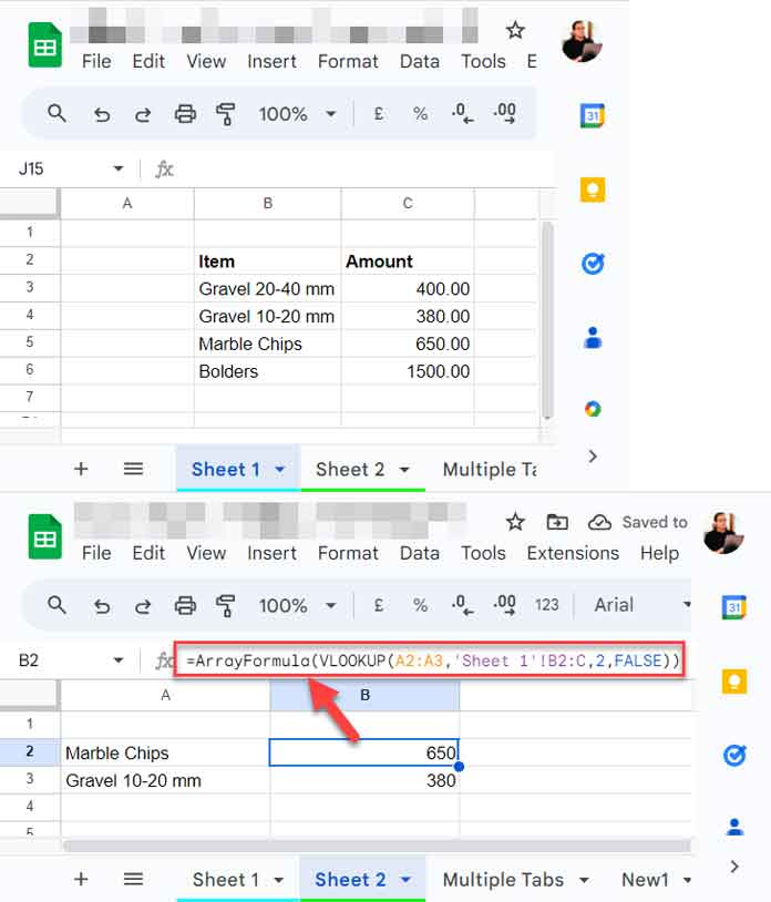
My sample data (lookup table) is in “Sheet 1.” The range is B2:C6, where B1:C1 contains the field labels.
| Item | Unit Price |
| Gravel 20-40 mm | 400.00 |
| Gravel 10-20 mm | 380.00 |
| Marble Chips | 650.00 |
| Bolders | 1500.00 |
I want to Lookup this table from another sheet.
For example, when I enter “Marble Chips” in cell A2 in “Sheet 2,” I want to get the unit price of that item in cell B2 in that sheet from “Sheet 1.”
Here is how to perform VLOOKUP from another sheet in Google Sheets.
B2 Formula:
=VLOOKUP(A2,'Sheet 1'!B2:C,2,FALSE) search_key: A2
range: ‘Sheet 1’!B2:C
index: 2
is_sorted: FALSE
Key Points
- The function will search for the
search_key, i.e., “Marble Chips,” in the first column of therange. - It returns the result from the
indexcolumn. - The
is_sortedmust be FALSE for an exact match. Specify TRUE only in a sorted range.
Can I VLOOKUP from another sheet and return the price of more than one item in one go?
Yep! We can use the ARRAYFORMULA with VLOOKUP for that, and here is an example.
=ArrayFormula(VLOOKUP(A2:A3,'Sheet 1'!B2:C,2,FALSE))
The above approach won’t work with VLOOKUP across multiple sheets. There we should first combine ranges from different sheets. Below you can find those tips.
VLOOKUP Across Multiple Sheets in a Workbook in Google Sheets
How do we perform VLOOKUP across multiple sheets in Google Sheets?
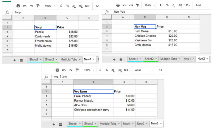
Assume we have price lists of soups, nonveg, and veg items in the range 'New1'!B3:C, ‘New2'!B3:C, and 'New3'!B3:C in a workbook.

I have a search key (“Crab Masala”) in ‘Search’!A1 (another sheet in that workbook).
I want to look through the ranges to find the matching row of the search key and return the value from the “Price” column.
In other words, I want to perform VLOOKUP across multiple sheets in a Google Sheets file.
How do we do it?
Just simple! Combine those ranges below one another using VSTACK to get a combined range.
With VSTACK, we may additionally require to perform some data cleaning to remove blank rows and thus enhance the performance of our VLOOKUP formula.
Here is the formula to use as the range in VLOOKUP.
Combined Range:
=LET(
     appended,
     VSTACK('New1'!B3:C,'New2'!B3:C,'New3'!B3:C),
     FILTER(
          appended,
          TRIM(TRANSPOSE(QUERY(TRANSPOSE(appended),,9^9)))<>""
     )
)
I’ve combined three sheets. If you have more, specify them within the VSTACK; no need to make any other changes.
VLOOKUP Across Multiple Sheets:
I’ve bolded the above range in the following formula.
=LET(
     combined_range,
     LET(
          appended,
          VSTACK('New1'!B3:C,'New2'!B3:C,'New3'!B3:C),
          FILTER(
               appended,
               TRIM(TRANSPOSE(QUERY(TRANSPOSE(appended),,9^9)))<>""
          )
     ),
     VLOOKUP('Search'!A1,combined_range,2,FALSE)
)range: combined_range (It’s the name of the bolded part of the formula. Used LET to assign that name)
search_key: ‘Search’!A1 (contains “Crab Masala”)
index: 2
is_sorted: FALSE
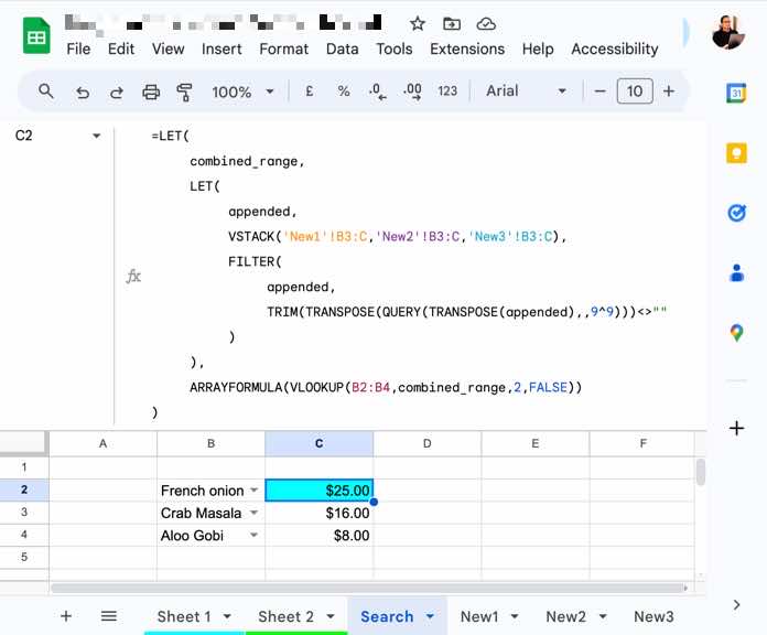
What about specifying search keys in a cell range and performing VLOOKUP across multiple sheets in Google Sheets?
Please see the below formula and screenshot.
=LET(
     combined_range,
     LET(
          appended,
          VSTACK('New1'!B3:C,'New2'!B3:C,'New3'!B3:C),
          FILTER(
               appended,
               TRIM(TRANSPOSE(QUERY(TRANSPOSE(appended),,9^9)))<>""
          )
     ),
     ARRAYFORMULA(VLOOKUP(B2:B4,combined_range,2,FALSE))
)
If you have several sheets to combine in a workbook, use my COPY_TO_MASTER_SHEET named function.


May I ask if the length of all the tab has to be the same?
Hi, Chi,
It’s not an issue. You can use sheets with a different number of total rows.
Tip:
Instead of using multiple sheets range as below;
{'New1'!B3:C;'New2'!B3:C;'New3'!B3:C}you can use the below formula to improve your Sheets’ performance.
query({'New1'!B3:C;'New2'!B3:C;'New3'!B3:C},"Select * where Col1 is not null")Thanks for your help with this, really came in handy!