There are two options to remove leading, trailing, and repeated space characters in text in Google Sheets: using the TRIM function or the built-in Trim Whitespace command.

Both have their pros and cons. The TRIM function is typically used in combination with other functions, such as SPLIT, for more detailed text processing. The built-in Trim Whitespace command is useful for quickly removing extra spaces from the source data.

Syntax of the TRIM Function:

TRIM(text)

• text: The string or reference to a cell or array containing the string(s) to be trimmed. When using it in an array, you must use the ARRAYFORMULA function, and the syntax would be:

=ARRAYFORMULA(TRIM(text))

How to Remove Extra Spaces in Google Sheets

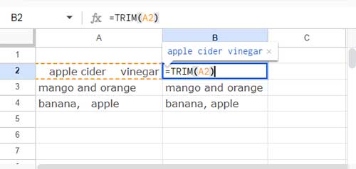
Cell A2 contains the following text:

 apple cider   vinegar 

If you use the formula =TRIM(A2) in cell B2, it will return “apple cider vinegar,” removing all extra space characters from the string.

If you have more text in the column, you can drag the fill handle of B2 down or use the TRIM function as an array formula:

=ArrayFormula(TRIM(A2:A))

Before entering the array formula, make sure that B2:B is blank; otherwise, the formula may break.

If you do not want the result in a new cell, use the built-in command:

1. Navigate to cell A2 or select the range A2:A.
2. Click Data > Data Clean-Up > Trim Whitespace.
3. Click OK on the notification window that appears.

The Most Effective Combo: TRIM and SPLIT Functions

When you split a delimited text string, you might find leading spaces.

To illustrate, let’s split the following text string:

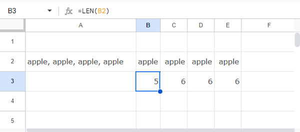
apple, apple, apple, apple

As you can see, each “apple” has five characters. Observe what happens when we split it.

Enter the following formula in cell B2, assuming the text is in cell A2:

=SPLIT(A2, ",")

This will split the text based on the comma delimiter, and the result will be displayed in cells B2 through E2.

To check the number of characters in each cell within the range B2:E2, enter the following LEN formula in B3 and drag it across:

=LEN(B2)

You’ll notice that it returns 5, 6, 6, 6 instead of 5 for all cells.

To correct this, wrap the SPLIT function with TRIM and apply ARRAYFORMULA, as SPLIT returns an array:

=ArrayFormula(TRIM(SPLIT(A2, ",")))

Why the TRIM Function Isn’t Removing All Space Characters in Google Sheets

If you still see whitespace after using the TRIM function or the Trim Whitespace tool, the characters might be tabs, carriage returns, or non-breaking spaces.

The TRIM function and the Trim Whitespace command in Google Sheets only remove standard spaces, not other characters like tabs, carriage returns, or non-breaking spaces.

In such cases, you can use a combination of the TRIM, REGEXREPLACE, AND SUBSTITUTE functions to remove extra whitespace characters.

How to Test It

To generate sample text for testing, enter the following formula in cell A2:

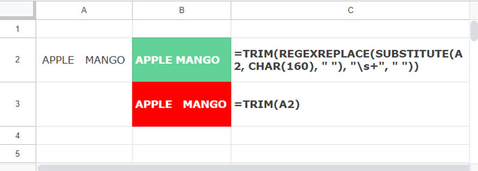
=CHAR(9)&"APPLE"&CHAR(13)&CHAR(160)&CHAR(32)&"MANGO"&CHAR(9)

This will produce text with extra spaces between the words, including tabs, carriage returns, regular spaces, and non-breaking spaces.

In cell B2, enter the following formula:

=TRIM(REGEXREPLACE(SUBSTITUTE(A2, CHAR(160), " "), "\s+", " "))

Where:

• SUBSTITUTE(A2, CHAR(160), " "): Replaces non-breaking spaces with regular spaces.
• REGEXREPLACE(…, "\s+", " "): Replaces all sequences of whitespace characters (spaces, tabs, carriage returns) with a single space.
• TRIM(…): Removes any leading and trailing spaces from the result.

Additional Tip: Removing Extra Spaces with Find and Replace in Google Sheets

When Should We Use the Find and Replace Tool to Remove Whitespace in Google Sheets?

You can use the TRIM function or the Data > Data Clean-up > Trim Whitespace option to remove extra whitespace in specific ranges within a sheet. However, if you want to apply this to all sheets in a Google Sheets file, you would need to do so individually for each sheet.

In such cases, the Find and Replace command becomes very useful. You can use it within a specific range, a single sheet, or across multiple sheets. However, I recommend making a copy of your sheet and testing the command there first.

Here are the steps to follow:

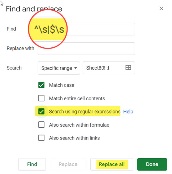
1. Click on Edit > Find and Replace.
2. In the Find field, enter the regular expression ^\s|$\s.
3. For Search, select one of the following options: All Sheets, This Sheet, or Specific Range. If you choose Specific Range, enter the range in the format, such as Sheet1!A1:A10.
4. Check the option “Search using regular expressions.”
5. Click the “Replace All” button. This will remove leading and trailing spaces from the text in the selected range or sheets.
6. Then, in the Find field, enter the regular expression \s+.
7. In the “Replace with” field, hit the space bar once.
8. Click “Replace All”. This will replace all consecutive occurrences of spaces with a single space (” “).
9. Click “Done.”

Resources

• Remove Whitespaces at the Beginning of a Newline in Google Sheets
• Padding Values with Spaces to Make Them Equal in Length in Sheets
• Copy-Paste Merged Cells Without Blank Rows/Spaces in Google Sheets