


")


")

")
")
 in Excel & Google Sheets")


Outliers can skew your averages, especially in sales, performance, or survey data. That’s where the TRIMMEAN function in Google Sheets comes in. Unlike AVERAGE, which includes all values, TRIMMEAN helps you exclude extreme values from both ends of your dataset—giving you a more accurate average.
What Is TRIMMEAN in Google Sheets?
The TRIMMEAN function in Google Sheets returns the mean (average) of a dataset after removing a certain percentage of values from both the top and bottom ends. It’s ideal when you want to exclude outliers—extremely high or low values—from your analysis.
Syntax:
TRIMMEAN(data, exclude_proportion)- data: The range or array of numeric values.
- exclude_proportion: The proportion of data to exclude, given as a decimal or percentage (between 0 and 1).
Example: If you set exclude_proportion = 0.1, it means 10% of the dataset will be removed—5% from the bottom and 5% from the top.
So if you have 100 data points, TRIMMEAN will:
- Exclude the lowest 5 and the highest 5 values.
- Calculate the mean of the remaining 90 values.
Why Use TRIMMEAN Instead of AVERAGE?
Let’s say you have the following sales data:
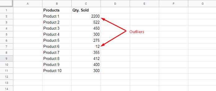
If you calculate the average using:
=AVERAGE(C2:C11)You’ll get 522.6, which is inflated due to the outliers 2200 and 12.
Now try:
=TRIMMEAN(C2:C11, 0.2)Or:
=TRIMMEAN(C2:C11, 20%)This excludes the two extreme values (20% total = 10% from each end) and gives you a much truer average of 376.75.
Conditional TRIMMEAN in Google Sheets
You can also apply conditions to your dataset using FILTER or QUERY.
Example 1: Using FILTER
=TRIMMEAN(FILTER(C2:C11, B2:B11 <> "Product 1"), 10%)This removes “Product 1” from the calculation, then trims 10% of the remaining data.
Example 2: Using QUERY
=TRIMMEAN(QUERY(B2:C11, "Select C where B <> 'Product 1'"), 10%)Same result, but powered by QUERY. You can add more conditions easily as your dataset grows.
When to Use TRIMMEAN in Real Life?
- Sales Reports: Remove unusually large or small orders.
- Survey Analysis: Ignore extreme responses.
- Project Durations: Remove anomalies from time estimates.
- Marketing Spend: Trim one-off campaign spikes.
Key Tips for Using TRIMMEAN
- Works best on datasets with more than 10 values.
- Adjust the proportion based on how extreme your outliers are.
- Use with FILTER or QUERY for conditional outlier exclusion.
- For weighted averages, use AVERAGE.WEIGHTED instead.
Conclusion
The TRIMMEAN function in Google Sheets is a better choice than AVERAGE when accuracy matters. It gives you a balanced average by removing extremes and works especially well for analytics, reporting, and large datasets.