In order to filter the top 3 values in each group in a pivot table report in Google Sheets, at present, we must use the custom formula field in the pivot editor. There is no pivot feature built-in for that.
This tutorial is meant to help you write the required formula to use in the custom formula field in the pivot table editor.
Actually, we can use the same formula (the formula that we are going to write) to filter the top ‘n’ (eg. top 1, 2, 3, 4, 5, 6, …10, and so on) in each group in the pivot table.
This tutorial contains two formulas to use in two different scenarios. I mean there are two types of reports.
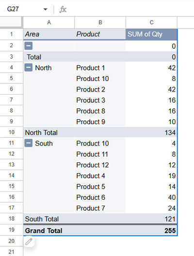
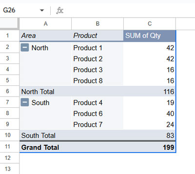
Please see the two images below for the two types of reports.
Report # 1 (Company-Wise Sales Summary of Top 3 Products from Each Group):
Report # 2 (Sales Summary of Top 3 Products from Each Group):
Pivot Reports and Sample Data Explained
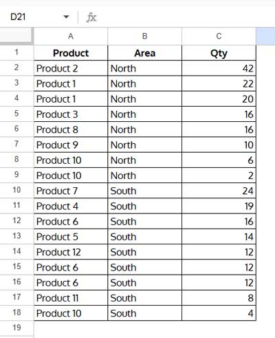
The sample data (in Report # 1 and Report # 2 above) is actually part of a sales report of crusher products.
There are two sales items (product sales).
- Black Sand 0-5 mm.
- Road Base – Crushed 0-50 mm.
The top 3 sales of each product are as follows.
- Black Sand 0-5 mm – 800, 700, and 600.
- Road Base – Crushed 0-50 mm – 800, 500, and 300.
We want to filter these top 3 values (sales) in each group in pivot table reports.
The first report has three columns in the sample data – Product, Company, and Sales.
So in the first pivot table report (Report # 1), there is a product column, a company column then top 3 sales (if any company appears more than one time in the top 3, then such values would be summed).
In the sample data for the second pivot table report (Report # 2), there are two columns – Product and Sales. So the pivot table report has only two columns – Product and top 3 sales summary.
Let’s see how to filter the top 3 sales values in each group as above in the pivot table report in Google Sheets.
How to Select Top 3 Values in Each Group in Pivot Table in Google Sheets
Before start writing the formula, let’s create the pivot table report. Then we can write and insert the formula within the corresponding filed in the pivot editor.
Pivot Report
I know you are well accustomed to creating pivot table reports in Google Sheets. Even though, I am including the steps below for newbies.
Here are the steps for the required pivot table that filters top ‘n’ values in each group (using the sample data in Report # 1 [please see the first image on the top]).
Steps:
- Select the range A1:C14. Then click Data > Pivot Table.
- Enable/select the “Existing sheet” as we are creating the report in the same sheet that contains the sample data.
- Select cell E2 and click “Create”.
You will get an ‘outline’ of the report and the pivot table editor panel will be opened on the screen.
Now follow the below steps to complete the report.
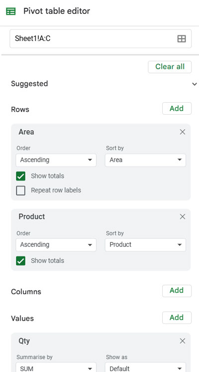
- On the editor panel, click “Add” against “Rows” and select “Product” (enable “Show total”).
- Repeat the above step and select “Company” (enable “Show total”)
- Click “Add” against “Values” and select “Sales”. In this last step, make sure that “SUM” is selected below “Summarize by” and “Show” as “Default”.
You will get the below pivot table report.
From this how to filter the top 3 values from each group, i.e. from “Black Sand 0-5 mm” and “Road Base – Crushed 0-50 mm”?
Logic to Filter the Top 3 Values from Each Group in the Pivot Table in Google Sheets
The logic is like this (if you find the logic difficult to understand, you can skip this logic part or read after completing writing the formula);
We will sort the product by sales in descending order. I mean sorting the “Product” column in ascending (A-Z) order and then by the “Sales” column in descending (Z-A) order. We will do this using a formula not physically within the sheet.
Then we will use my running count (RC) array formula to return the running count of “Products”.
Using an IF logical test we will return the values for the rows wherever the running count is LTE (less than or equal to) 3 or “N”.
The next step is to combine the corresponding “Product” and “Sales”.
Finally, we will Regexmatch the combined values in the original range A2:C within the pivot table.
We will follow the above logic to code a custom formula to use in the pivot table editor to filter the top 3 values in each group in the pivot table report in Google Sheets.
Coding Custom Formula for the Report # 1
I have a few running count tutorials. Here is the specific link to learn the same that is apt to our purpose – Cumulative Count of All the Items in a Sorted List.
Don’t get confused by “Sorted” in the link title. It’s actually about sorting “Products” not “Sales”.
Step # 1 – RC Formula
In cell D2, insert the below RC formula (we are just coding the formula within the worksheet to use in the pivot table editor later).
=ARRAYFORMULA(COUNTIFS(A2:A,A2:A,ROW(A2:A),"<="&ROW(A2:A)))
Result:
I have used a COUNTIFS-based ArrayFormula for RC. See the count restarts in the result when the “Product” changes.
Step # 2 – Running Count (RC) Sorting by Sales
This is the second step to filter the top 3 (“N”) sales in each group in the pivot table report in Google Sheets.
Here we are going to slightly modify the above formula to make the range sorted by “Product” in A-Z order and “Sales” in Z-A order.
Simply replace the A2:A (first two) in the formula with the following formula.
array_constrain(sort(A2:C,1,1,3,0),9^9,1)
The SORT formula sorts the first column in A2:C in ascending order and the last column in A2:C in descending order.
The Array_Constrain constrains the number of columns in A2:C to 1, i.e. A2:A.
Here is the formula after the said modification.
=ARRAYFORMULA(COUNTIFS(array_constrain(sort(A2:C,1,1,3,0),9^9,1),array_constrain(sort(A2:C,1,1,3,0),9^9,1),ROW(A2:A),"<="&ROW(A2:A)))
Step # 3 – Combine Product and Sales Based on Sorted RC
Generic Formula:
=If(step_2_result<=3,sorted_prodcut&sorted_sales,)
To get sorted_product use the below SORT formula.
array_constrain(sort(A2:C,1,1,3,0),9^9,1)
The formula for sorted_sales.
array_constrain(sort({C2:C,A2:A},2,1,1,0),9^9,1)
Here is the step # 3 formula as per the above generic formula.
=ArrayFormula(if(COUNTIFS(array_constrain(sort(A2:C,1,1,3,0),9^9,1),array_constrain(sort(A2:C,1,1,3,0),9^9,1),ROW(A2:A),"<="&ROW(A2:A))<=3,array_constrain(sort(A2:C,1,1,3,0),9^9,1)&array_constrain(sort({C2:C,A2:A},2,1,1,0),9^9,1),))
You just need to filter the rows in A2:C matching the above outputs in column D to select only the top 3 values in each Group in the pivot table in Google Sheets. Read on to know how to do that.
Step # 4 – Regex Match to Filter the Top “N” Values in Each Group in Google Sheets Pivot Table
The generic Regexmatch formula would be like this.
regexmatch(Product&Sales,step_3_result_as_regular_expression)
In this “Product” and “Sales” are filed labels (A1:A and C1:C). We can use field labels instead of array/range references in the Pivot Editor formula field.
The step_3_result (step # 3 formula result) should be formatted as a regular expression. TextJoin will do that.
See the highlighted part which is the added part to the step # 3 formula to form the regular expression.
Here is the much-awaited custom formula to filter the top 3 values group-wise in the pivot table in Google Sheets.
=regexmatch(Product&Sales,"^"&textjoin("$|^",1,ArrayFormula(if(not(len(A2:A)),,if(COUNTIFS(array_constrain(sort(A2:C,1,1,3,0),9^9,1),array_constrain(sort(A2:C,1,1,3,0),9^9,1),ROW(A2:A),"<="&ROW(A2:A))<=3,array_constrain(sort(A2:C,1,1,3,0),9^9,1)&array_constrain(sort({C2:C,A2:A},2,1,1,0),9^9,1),))))&"$")
How do I use this formula in the pivot table?
To insert the above formula that filters/selects the top 3 values in each group in the pivot table in Google Sheets, follow the below steps.
- Click cell E2 to enable the pivot editor panel.
- Scroll to the top of the editor and change the “Data range” A1:C14 to A1:C100 or up to the range that you want (you can include blank rows to accommodate future sales entries).
- Scroll down to the bottom of the panel and click “Add” against “Filter”.
- Select “Product” which is the primary group field.
- Click the drop-down (by default it may show “Showing all items”) and select Filter by Condition > Custom formula is.
- Insert the above formula and click “OK”.
That’s all!
Coding Custom Formula for the Report # 2
At the beginning of this post, I have shown you two types of reports. I have detailed Report # 1 (3 columns – Product, Company, and Sales) above.
In Report # 2 (2 columns – Product and Sales) we can use the above formula with some changes. Those changes are in Step # 2 and Step # 3.
Since we have two columns, we should change the sort range accordingly. That means, in step 2, here A2:A must be replaced by array_constrain(sort(A2:B,1,1,2,0),9^9,1)
.
Here in step # 3, the sorted_product will be array_constrain(sort(A2:B,1,1,2,0),9^9,1)
and sorted_sales will be array_constrain(sort({B2:B,A2:A},2,1,1,0),9^9,1)
.
There are no other changes. Here is the final formula (after incorporating the above-said changes) to use in the pivot table editor to filter the top 3 values in each group.
=regexmatch(Product&Sales,"^"&textjoin("$|^",1,ArrayFormula(if(not(len(A2:A)),,(if(COUNTIFS(array_constrain(sort(A2:B,1,1,2,0),9^9,1),array_constrain(sort(A2:B,1,1,2,0),9^9,1),ROW(A2:A),"<="&ROW(A2:A))<=3,array_constrain(sort(A2:B,1,1,2,0),9^9,1)&array_constrain(sort({B2:B,A2:A},2,1,1,0),9^9,1),)))))&"$")
How to Filter Top “N” Instead of Top 3 in Each Group in Pivot Table?
In the formula change <=3 to <=n. In this replace “n” with 5 or any number of rows that you want to filter from each group in the pivot table.
That’s all. Enjoy!
Resources: