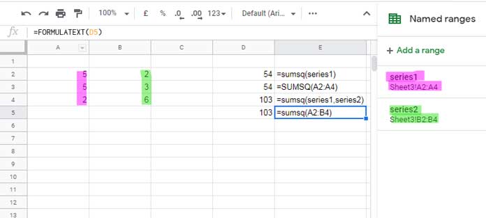
The SUMSQ is a math function in Google Sheets that returns the sum of the squares of a series of values.
In this post, you’ll learn how to use the SUMSQ function in detail. I’ll also show you a few alternative formulas you can use instead — especially for conditional scenarios where SUMSQ doesn’t support criteria directly.
Let’s begin.
SUMSQ Function in Google Sheets – Syntax, Arguments, and Examples
Syntax:
SUMSQ(value1, [value2, ...])Arguments explained:
- value1 – The first number or array whose squares to add.
- value2, … – Additional numbers or arrays whose squares to add to the first one.
Only the first argument is required. The rest are optional.
Examples
Here’s a simple example using just one number:
=SUMSQ(5)This returns 25, which is just 5². So, if you use only one number, SUMSQ just returns its square.
Now here’s one with multiple arguments:
=SUMSQ(5, 5, 2)This equals 5² + 5² + 2², or 25 + 25 + 4 = 54.
Using Cell References and Named Ranges
You’re not limited to hardcoding numbers — the SUMSQ function also accepts cell references, ranges, and named ranges.
Examples:
=SUMSQ(series1)                // 'series1' is a named range
=SUMSQ(A2:A4)                  // a vertical range
=SUMSQ(series1, series2)       // two named ranges
=SUMSQ(A2:B4)                  // a 2D array
A Few Notes
- Text and Boolean values (like TRUE/FALSE) are ignored.
- If any referenced cell has an error, SUMSQ will return that error.
- While some documentation mentions a 30-argument limit, in practice Google Sheets allows an arbitrary number of arguments.
Sum of Squares Without Using SUMSQ
You don’t always need the SUMSQ function to calculate the sum of squares in Google Sheets. You can use other formulas involving POWER, POW, or even the caret symbol ^.
Let’s say this is your data:
| A | B |
|---|---|
| 3 | 10 |
| 4 | 1 |
| 2 | 5 |
The following formula will give the sum of squares:
=SUMSQ(A1:B3)Now, here are some alternatives using other functions:
1. Using POWER:
=SUMPRODUCT(POWER(N(A1:B3), 2))2. Using POW:
=SUMPRODUCT(POW(N(A1:B3), 2))3. Using ^:
=SUMPRODUCT(N(A1:B3)^2)A Key Difference to Note
These formulas treat TRUE as 1, while SUMSQ ignores Boolean values. That’s why I’m showing you these options — in case that difference matters in your dataset.
Technically, you can tweak the alternatives to ignore TRUE, but there’s not much reason to go that far unless you’re dealing with mixed data.
Is There a SUMSQIF or SUMSQIFS Function in Google Sheets?
No — Google Sheets doesn’t have SUMSQIF or SUMSQIFS. And I doubt it ever will. But that doesn’t mean you can’t do a conditional sum of squares.
Here’s how you can handle it with FILTER or QUERY.
Using FILTER
Say column A has numbers and column B has “Yes” or “No”:
=SUMSQ(FILTER(A1:A, B1:B = "Yes"))This will return the sum of squares in column A, but only for rows where column B is “Yes”.
Using QUERY
Here’s the same logic using QUERY:
=SUMSQ(QUERY(A1:B, "SELECT A WHERE B='Yes'"))If you’re comfortable with FILTER or QUERY, creating conditional SUMSQ formulas is pretty straightforward — even with multiple conditions.
That’s It!
Now you know how to use the SUMSQ function in Google Sheets, plus a few handy alternatives. Whether you’re working with raw numbers, ranges, or even conditional logic, there’s always a way to get the sum of squares you’re after.


