


")


")

")
")
 in Excel & Google Sheets")


If you’ve ever found yourself manually summing every few columns or rows in Google Sheets—quarterly totals, weekly data, or groupings of N values—there’s a better way. You can build dynamic formulas that do the work for you. In this post, I’ll show you how to sum every N cells to the right (across columns) or to the bottom (down rows) using flexible formulas that grow with your data.
We’ll cover both traditional drag-down formulas and modern array formulas—so whether you prefer a simple OFFSET approach or the flexibility of WRAPROWS, WRAPCOLS, and LAMBDA, you’ll find a method that fits your workflow.
Sum Every N Cells to the Right in Google Sheets
Example Data Setup for Summing Across Columns
Let’s say you have monthly sales data in row 3 from column B to column M (range B3:M3). You want to group them into quarters by summing every 3 columns.
1. Using a Non-Array Formula (Drag Right)
Start with this formula in cell B6 and drag it to the right:
=SUM(OFFSET($B$3, 0, (COLUMN() - COLUMN($B$3)) * 3, 1, 3))
Want to group every 4 columns instead of 3? Just change both instances of 3 in the formula to 4.
What’s Happening:
$B$3is your starting point.- The formula dynamically shifts right using
(COLUMN() - COLUMN($B$3)) * 3, which evaluates to 0, 3, 6, etc., as you drag it across. - OFFSET then pulls a 1-row, 3-column slice to sum.
Heads-up: If you paste this somewhere other than column B, make sure to adjust COLUMN($B$3) to match your current column.
2. Using a Dynamic Array Formula (No Dragging Needed)
Here’s the cleaner, one-formula alternative:
=BYCOL(WRAPCOLS(B3:M3, 3, 0), LAMBDA(c, SUM(c)))This one’s pretty slick:
1. WRAPCOLS splits the row into chunks of 3.
| 5000 | 7500 | 6000 | 8000 |
| 5000 | 7500 | 6000 | 8000 |
| 5000 | 7500 | 6000 | 0 |
2. BYCOL applies a SUM to each chunk.
Change the 3 to any N value to sum every N columns.
Sum Every N Cells to the Bottom in Google Sheets
Now let’s look at vertical data—like daily totals or survey responses stored in a single column. You want to sum every N rows.
Example Data Setup for Summing Down Rows
Assume values are in D2:D13. You want to sum every 3 rows and output each total in a separate cell.
1. Using a Non-Array Formula (Drag Down)
Insert this formula in H2, then drag it down:
=SUM(OFFSET($D$2, (ROW() - ROW($D$2)) * 3, 0, 3))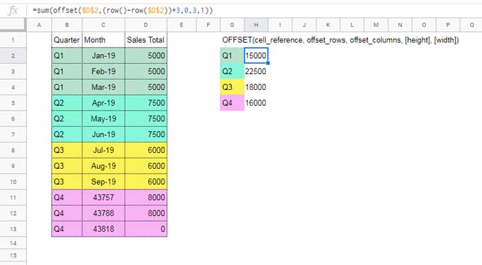
Again, adjust the 3 if you want different-sized groups.
How It Works:
$D$2is the top of your data.(ROW() - ROW($D$2)) * 3returns 0, 3, 6, 9… as you move down.- OFFSET shifts downward and sums the next 3 rows.
If you’re placing the formula in a different row (e.g., starting from row 3 instead of row 2), make sure to update the reference to ROW($D$3) in the formula so it matches the row where you’re placing it. This ensures the row offset calculation remains accurate.
2. Using a Dynamic Array Formula (All at Once)
No dragging needed with this modern formula:
=BYROW(WRAPROWS(D2:D13, 3, 0), LAMBDA(r, SUM(r)))Here’s what’s going on:
1. WRAPROWS splits your vertical list into 3-row groups.
| 5000 | 5000 | 5000 |
| 7500 | 7500 | 7500 |
| 6000 | 6000 | 6000 |
| 8000 | 8000 | 0 |
2. BYROW sums each group.
You guessed it—just change the 3 to whatever N you need.
Wrapping Up
Whether you’re summing by column or by row, the dynamic formulas above can save you from repetitive work. You’ve now got:
- A drag-down (or right) solution using
OFFSET - A dynamic array solution using
WRAPROWS,WRAPCOLS, andLAMBDA
These flexible options make it easy to sum every N cells to the right or bottom in Google Sheets—no helper columns or manual effort required.
Hi, Prashanth,
Why do am I getting Error stating;
“OFFSET evaluates to an out of bounds range”
=SUM(OFFSET(Days!$X$3,0,(COLUMN()-column(Days!$X$3))*5,1,5))Please do help.
Please check the “Usage Note 1” especially the first point.
You are inserting the formula in cell B8, i.e. in column B. So the formula must be;
=SUM(OFFSET(Days!$X$3,0,(COLUMN()-column(Days!$B$3))*5,1,5))