The Pivot table is quite useful for summarizing and reorganizing data in Google Sheets and as well as in other Spreadsheet applications. If you are using this functionality, at some point in time, you may want to sort the Grand Total columns at the bottom of the Pivot table report.

It’s possible and easy to sort the Pivot table Grand Total columns in Google Sheets. You can find all the necessary pieces of information related to this below.

The steps are not the same in Google Sheets and Excel. So, if you are an Excel user, who switched to Google Sheets, you may take time to find the required steps in Google Sheets. So I hope that you will find this tutorial helpful.

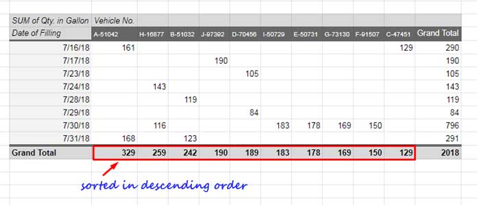
Descending Order:

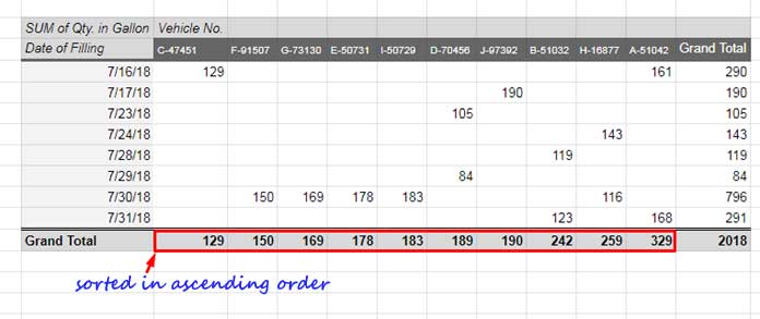
Ascending Order:

To sort the Pivot table Grand Total columns in ascending or descending order, you must change the settings in your Pivot table editor in the “Columns” field.

Steps to Sort Pivot Table Grand Total Columns

Before coming to that step, let me show you how to create the above Pivot report (without sorting).

Sample Data:

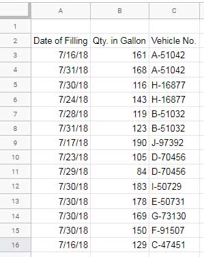
First, select the data (A2:C16) and then go to the menu Insert > Pivot table.

Select “New sheet” or “Existing sheet” (you might want to select the ‘insert cell’ in this case) and click the Create button.

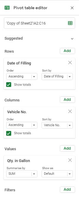
Inside the Pivot table editor panel, you must add (1) Rows, (2) Columns, and (3) Values.

In our data, there are three columns. Let me show you how to include these three columns in the Pivot table. You can jump to the screenshot skipping the 3 points below.

1. Values: The values to sum are in column B (“Qty. in Gallon”). So add this column to the Values field and choose the aggregate function from the drop-down. I am choosing SUM here.
2. Rows: I am adding the data in column A (“Date of Filling”) in this field.
3. Columns: Now, add the last column C (“Vehicle No.”) in the Columns field.

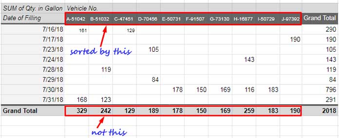
Our Pivot Table report is ready. Check the columns. It’s by default sorted based on the field labels (Vehicle No.).

Sorting Grand Total Columns in Descending or Ascending Order

To sort the Grand Total columns (the total row at the bottom) in descending or ascending order, you must edit the “Column” field inside the Pivot table editor.

Note:- If the Pivot table editor is off (closed), hover your mouse pointer over the Pivot table report. Will pop up a pencil/pen icon at the bottom corner (left-hand side). Click on it to open the panel.

Just have a look at the “Columns” field. You can see that the default sorting is “Vehicle No.” in ascending order.

You must change it to sort by “SUM of Qty. in Gallon…” (the field used in “Values” with aggregation SUM) and then select “Grand Total.”

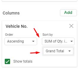
This setting will sort the above Pivot table Grand Total columns in ascending order. Just change “Ascending” to “Descending” (see the above image) to change the pivot table sort order.

Tip: We can apply the same to the Rows field (Date of Filling) total.

That’s all. Enjoy!

Additional Resources

1. How to Use GETPIVOTDATA Function in Google Sheets.
2. Create an Age Analysis Report Using Google Sheet Pivot Table.
3. Month Wise Pivot Table Report in Google Sheets Using Date Column.
4. Group Dates in Pivot Table in Google Sheets (Month, Quarter, and Year).
5. Adding Calculated Field in Pivot Table in Google Sheets.
6. Drill Down in Pivot Table in Google Sheets (Date Field).