


")


")

")
")
 in Excel & Google Sheets")


When working with grouped data in Google Sheets—like tasks under a project, assignments for a student, or quality checks for a product—you might want to display only the groups where every row meets a specific condition. For example, you may want to show only those projects where all tasks are marked as “Completed,” or only students who have submitted every assignment.
In this tutorial, you’ll learn how to show only complete groups in Google Sheets using formulas—meaning, groups where all rows meet a certain condition. This helps clean up your reports, focus on finalized work, and create more meaningful dashboards or summaries.
Let’s dive into a real-world use case to see how it works.
Sample Data
Consider the following dataset of student assignments and their completion status. Each student appears multiple times—once for each assignment—making them a grouped entry.
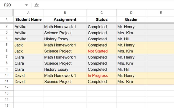
Your goal is to filter only those students who have completed all of their assignments—in other words, to show only complete groups in Google Sheets, where every row within a group meets the condition "Completed".
Formula to Show Only Complete Groups
To show only complete groups where all statuses are marked "Completed", enter the following formula in cell F2:
=FILTER(A2:D, ISNA(XMATCH(A2:A, UNIQUE(FILTER(A2:A, C2:C<>"Completed")))))Example Output
| Student Name | Assignment | Status | Grader |
| Advika | Math Homework 1 | Completed | Mr. Henry |
| Advika | Science Project | Completed | Mrs. Kim |
| Advika | History Essay | Completed | Mr. Hill |
| Clara | Math Homework 1 | Completed | Mr. Henry |
| Clara | Science Project | Completed | Mrs. Kim |
| Clara | History Essay | Completed | Mr. Hill |
In this example, Advika and Clara are the only students who have completed all their assignments. The formula filters out the rest.
Formula Explanation
Let’s break down how this formula works to filter complete groups in Google Sheets:
=FILTER(A2:D, ISNA(XMATCH(A2:A, UNIQUE(FILTER(A2:A, C2:C<>"Completed")))))1. FILTER(A2:A, C2:C<>"Completed")
This returns a list of student names where at least one assignment is not marked "Completed". These are the incomplete groups.
2. UNIQUE(...)
Removes duplicates from that list, leaving only unique student names who have incomplete tasks.
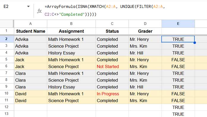
3. XMATCH(A2:A, ...)
Checks each student name in the original data against the list of incomplete students. If there’s a match, it returns a number; otherwise, it returns #N/A.
4. ISNA(...)
This turns the #N/A (i.e., students not in the incomplete list) into TRUE, and all others into FALSE. So only fully complete groups are marked TRUE.
5. FILTER(A2:D, ...)
Finally, this filters and returns the rows where ISNA is TRUE—in other words, rows belonging to students who completed all assignments.
Why This Is Useful
This method to show only complete groups in Google Sheets is helpful in many real-world scenarios:
- Education: Display only students who submitted all required assignments.
- Sales: Show only leads who completed every qualification step.
- Manufacturing: Filter product batches where all quality checks passed.
- Event Planning: Display teams who finished every preparation task.
By focusing only on complete data groups, you can reduce noise, streamline reporting, and highlight what’s ready for the next step.
Make It Dynamic for Dashboards
If you’re building a dynamic dashboard or report that updates automatically, you can make the group filter responsive to a selected status (e.g., "Completed" or "In Progress").
Step-by-step:
- Use a dropdown in cell
E1with your desired status. - Replace hardcoded
"Completed"in the formula with a reference toE1.
Dynamic Formula Example:
=LET(
   data, A2:D,
   categoryCol, A2:A,
   statusCol, C2:C,
   status, E1,
   FILTER(data, ISNA(XMATCH(categoryCol, UNIQUE(FILTER(categoryCol, statusCol<>status)))))
)
Now your sheet will dynamically filter complete groups based on the status selected in cell E1. This is especially useful in dashboards or interactive reports where users want to focus on different types of completion statuses.
Related Resources
Here are a few related tutorials that complement this technique: