")
")


")


")

")
")
 in Excel & Google Sheets")


The ROUND function isn’t supported directly inside a Google Sheets QUERY. So how do we round numbers in a Google Sheets Query? Is it even possible?
As far as I know, there’s no QUERY clause that can round a number directly. But there are two ways around this.
The FORMAT clause in QUERY lets us visually round numbers—that is, it makes them look rounded. But if you want to actually round numbers (not just format them), I’ve got a handy workaround.
In this post, I’ll show both approaches to round numbers in Google Sheets Query: one using FORMAT, and the other using functions like ROUND outside of QUERY.
If you haven’t yet seen my post on formatting numbers in Query, check that out here:
How to Format Date, Time, and Number in Google Sheets Query
Rounding in Query Using the Format Clause
I’ve got two examples for how to round numbers in a Google Sheets Query using FORMAT. The first example shows how to visually round a column from your data. The second rounds the output of a calculation.
Example 1: Visually Rounding Numbers and Percentages
Here’s a sample table showing gold price performance in Europe over various time frames, as of 25/07/2020.
| Change | Amount | % |
|---|---|---|
| 12 months | 361.67 | 28.47% |
| 6 months | 199.65 | 13.94% |
| 1 month | 62.86 | 4.01% |
The actual data isn’t important—it’s just for demonstration. We’re rounding the second and third columns in this data using QUERY.
I’ve selected the range A1:C so we can format both numbers and percentages in one go. Column B has numeric values (amounts), and column C shows percentage changes.
=QUERY(A1:C, "SELECT * FORMAT B '#', C '#%'")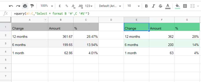
This is how we can format numbers in Google Sheets Query to look rounded.
Note: It’s only visual rounding.
Click into cell F2 or G2, and the formula bar will still show 361.67 (not 362) and 28.47% (not 28%).
Example 2: Rounding a Calculated Column with FORMAT
Now let’s say you want to multiply two columns—like B and C—and round the result.
=QUERY(A1:C, "SELECT A, B, C, B*C LABEL B*C 'Amt' FORMAT B*C '0'", 1)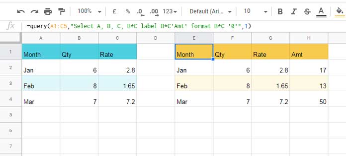
In the SELECT clause, I’ve included columns A, B, C, and B*C. Then I used the FORMAT clause to visually round the output column.
Since B*C creates a new column, I also labeled it using the LABEL clause.
Check out: Understand the Label Clause in Google Sheets Query
Rounding in Query Using the ROUND Function
As mentioned earlier, the two examples above only format the numbers to appear rounded. If you want to actually round values in your Query result, here’s the workaround.
We’ll build a virtual table using ARRAYFORMULA, apply ROUND before passing it to the QUERY function, and get truly rounded output.
Formula Based on Example #1
If you’re following Example #1, here’s how you can modify the formula to truly round numbers in QUERY.
=ARRAYFORMULA(
  QUERY(
    HSTACK(A1:A, ROUND(B1:B), ROUND(C1:C, 2)),
    "SELECT * WHERE Col1 IS NOT NULL LABEL Col2 'Amount', Col3 '%'"
  )
)
Here, we’re building a new table using HSTACK:
- Column A is text (no rounding needed)
- Column B is rounded using
ROUND(B1:B) - Column C is rounded to two decimal places using
ROUND(C1:C, 2)
You can also use ROUNDUP() or ROUNDDOWN() depending on your needs.
If you’re curious why percentages like C1:C use ROUND(..., 2), I’ve explained that here:
How to Round Percentage Values in Google Sheets
Formula Based on Example #2
Here, we want to round a calculated column like B*C in the Query result. We’ll name the formula using LET, extract and round the target column, then recombine everything using HSTACK.
Here’s the original formula:
=QUERY(A1:C, "SELECT A, B, C, B*C WHERE A IS NOT NULL", 1)Note: We’ve added the WHERE A IS NOT NULL clause to filter out empty rows. Without this condition, blank rows in the data could return 0 when performing calculations and rounding.
Output:
| Month | Qty | Rate | product(QtyRate) |
| Jan | 6 | 2.8 | 16.8 |
| Feb | 8 | 1.65 | 13.2 |
| Mar | 7 | 7.2 | 50.4 |
Let’s break down the workaround to round the last column.
Step 1: Use LET() to name the Query result
=LET(qry, QUERY(A1:C, "SELECT A, B, C, B*C WHERE A IS NOT NULL", 1), qry)Step 2: Separate columns 1–3 and column 4
=LET(
  qry, QUERY(A1:C, "SELECT A, B, C, B*C WHERE A IS NOT NULL", 1),
  cols1_3, CHOOSECOLS(qry, 1, 2, 3),
  cols4, CHOOSECOLS(qry, 4),
  HSTACK(cols1_3, cols4)
)
This setup replicates the original Query output.
Step 3: Apply ROUND() to the calculated column
=LET(
  qry, QUERY(A1:C, "SELECT A, B, C, B*C WHERE A IS NOT NULL", 1),
  cols1_3, CHOOSECOLS(qry, 1, 2, 3),
  cols4, CHOOSECOLS(qry, 4),
  HSTACK(cols1_3, ARRAYFORMULA(IFERROR(ROUND(cols4, 2), "Amt")))
)
Output:
| Month | Qty | Rate | Amt |
| Jan | 6 | 2.8 | 17 |
| Feb | 8 | 1.65 | 13 |
| Mar | 7 | 7.2 | 50 |
That’s it! This formula rounds numbers in a Google Sheets Query—not just visually, but actually.
Wrap-Up: Rounding Numbers in Google Sheets Query
This workaround is super useful when you need to round numbers in Google Sheets Query results instead of just formatting them. Whether it’s a raw data column or a calculated one, you’ve got flexible ways to round your numbers cleanly.
Enjoy!