Rotate Tasks Automatically in Google Sheets (Step-by-Step Tutorial)

When you have n members sharing tasks and want to rotate those tasks automatically, you can use a dynamic, formula-based approach in Google Sheets. Instead of manually reassigning tasks each day, week, or cycle, the formula shifts the task order automatically.

To do that, we use a combination of a circulant matrix and XLOOKUP. For example, if you have 5 tasks to share among 5 people and rotate them continuously, the first step is learning how to generate a 5×5 circulant matrix in Google Sheets.

Once you build the circulant matrix, you can use XLOOKUP to assign tasks dynamically—achieving automatic task rotation without scripts or manual editing.

Table of Contents

Step 1 — Arrange the Task List

Assume you have the following tasks:

Cleaning Kitchen
Vacuuming
Trash & Recycling
Groceries
Bathroom Cleaning

Enter them into a column, for example:

A2:A6

Step 2 — Generate the Circulant Matrix (Rotated Sequence Matrix)

You can use either the MAKEARRAY function or the SEQUENCE-based approach to generate the circulant matrix in Google Sheets. We’ll begin with SEQUENCE, and then show the MAKEARRAY alternative.

Formula using SEQUENCE

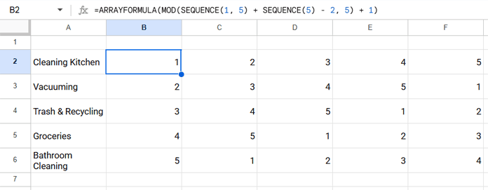
Enter the following formula in cell B2:

=ARRAYFORMULA(MOD(SEQUENCE(1, 5) + SEQUENCE(5) - 2, 5) + 1)

This creates a rotated sequence matrix like:

Example of a 5×5 rotated sequence matrix generated with a formula in Google Sheets

Alternative using MAKEARRAY

=MAKEARRAY(5, 5, LAMBDA(r, c, MOD(c + r - 2, 5) + 1))

Both formulas produce the same circulant matrix structure.

Step 3 — Use XLOOKUP to Rotate Tasks Automatically

Once you have the circulant matrix, you can lookup task names dynamically using XLOOKUP.

Enter this formula into cell H2:

=ARRAYFORMULA(XLOOKUP(B2:F6, SEQUENCE(5), A2:A6))

Automatic task rotation output after applying XLOOKUP formula in Google Sheets

This assigns tasks based on the rotated numbers and generates the automatic rotating task schedule.
Here:

Circulant matrix numbers (B2:F6) are the lookup values
SEQUENCE(5) is the lookup range
A2:A6 is the task list

Step 4 – Assign Members to Rotating Tasks

Enter member names in column G and the days/weeks in row 1.

Task rotation table showing member names and daily or weekly task assignments in Google Sheets

That’s it — you’ve now successfully set up automatic task rotation among members in Google Sheets.

All-in-One Dynamic Formula

If you want a single formula that counts the tasks, builds the rotating matrix, and assigns tasks in one step, use this version:

=ARRAYFORMULA(LET(list, TOCOL(A2:A, 1), n, COUNTA(list), XLOOKUP(MOD(SEQUENCE(1, n) + SEQUENCE(n) - 2, n) + 1, SEQUENCE(n), list)))

If your task list is in a different range, replace A2:A accordingly.

FAQ

1. Can I use this method for more or fewer tasks?

Yes. The formulas dynamically adapt to any number of items as long as ROWS = COLUMNS. The dynamic version automatically counts items.

2. Does this work for rotating shifts, chores, or duties?

Absolutely. This is a common method for rotating cleaning rosters, work shifts, group duties, study teams, and similar.

3. Do I need Apps Script or macros?

No — everything works using standard Google Sheets formulas. No scripts required.

4. What is a circulant matrix?

A circulant matrix is a matrix where each row is a cyclic shift of the previous one. It’s ideal for rotating sequences.

Conclusion

Using a circulant matrix combined with XLOOKUP is an elegant way to rotate tasks automatically in Google Sheets. It eliminates manual editing and keeps task assignment fair and balanced. Whether you’re organizing household chores, employee shifts, classroom responsibilities, or collaborative project duties, this approach is flexible and scalable.

Download the example sheet, try the formulas, and adapt them to your own rotating task schedule.

Get the Example Sheet

If you have suggestions or need improvements for your specific use case, feel free to ask in the comments.