Sometimes you may need to replace every nth delimiter in a string in Google Sheets — whether it’s a comma, an asterisk, or another separator. This can be handy for grouping items, formatting text for better readability, or even creating dynamic formulas like QUERY strings.
Fortunately, Google Sheets offers powerful functions like REGEXREPLACE that let you do this without manual edits.
Why Replace Every Nth Delimiter?
Here are a few scenarios where replacing every nth delimiter can be useful:
- Grouping data — e.g., grouping every 2 or 3 names together.
- Formatting formulas — like turning a repetitive multiplication pattern into an addition formula.
- Data preparation — breaking or marking sections in a long delimited string for later splitting.
Example 1: Replace Every Nth Delimiter for Grouping
Let’s start with a basic use case — grouping every 2 names from a comma-delimited string.
Sample data (A2):
Ben, John, Samuel, Megan, Joel, Edith, Diane, Teresa, Helen, Frank, Pauline, Mike
We want to create groups of two names separated by |:
Formula:
=REGEXREPLACE(
  REGEXREPLACE(A2,"(\,.*?){2}","$0|"),
  "\,\|"," |"
)
Output:
Ben, John | Samuel, Megan | Joel, Edith | Diane, Teresa | Helen, Frank | Pauline, Mike
Note: In the formula, the number inside { } (here {2}) represents the nth delimiter to replace. For example, use {3} to target every 3rd delimiter, {4} for every 4th, and so on.
Now, if you want to split these groups into rows:
=ARRAYFORMULA(TRIM(TRANSPOSE(SPLIT(
REGEXREPLACE(
  REGEXREPLACE(A2,"(\,.*?){2}","$0|"),
  "\,\|"," |"
), " |", FALSE))))
Output:
Ben, John
Samuel, Megan
Joel, Edith
Diane, Teresa
Helen, Frank
Pauline, Mike
Pro Tip:
For grouping specifically, you can also skip regex and use WRAPROWS like this:
=ARRAYFORMULA(
 LET(group, WRAPROWS(SPLIT(A2, ", "), 2),
 CHOOSECOLS(group, 1)&", "&CHOOSECOLS(group, 2))
)
Example 2: Replace Every Nth Delimiter to Create a Dynamic QUERY String
Now let’s look at a more advanced example — creating a dynamic aggregation part of a QUERY formula.
Sample Data
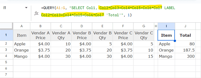
| Item | Vendor A Price | Vendor A Qty | Vendor B Price | Vendor B Qty | Vendor C Price | Vendor C Qty |
|---|---|---|---|---|---|---|
| Apple | $4.00 | 10 | $4.00 | 5 | $4.00 | 5 |
| Orange | $3.75 | 20 | $3.75 | 20 | $3.75 | 10 |
| Mango | $4.00 | 30 | $4.00 | 30 | $4.00 | 15 |
The standard query might look like:
=QUERY(A1:G, "SELECT Col1, Col2*Col3+Col4*Col5+Col6*Col7 LABEL Col2*Col3+Col4*Col5+Col6*Col7 'Total'", 1)
Instead of typing Col2*Col3+Col4*Col5+Col6*Col7 manually, we can generate it dynamically.
Step 1: Generate a Multiplication String
=ARRAYFORMULA(TEXTJOIN("*",TRUE,"Col"&SEQUENCE(1,6,2)))Output:
Col2*Col3*Col4*Col5*Col6*Col7
Step 2: Replace Every Second * with a +
Here’s where we use REGEXREPLACE to replace every nth delimiter (in this case, every 2nd asterisk) with a plus sign:
=REGEXREPLACE(
  REGEXREPLACE(
    ARRAYFORMULA(TEXTJOIN("*",TRUE,"Col"&SEQUENCE(1,6,2))),
    "(\*.*?){2}","$0+"
  ),
  "\*\+","+"
)
Output:
Col2*Col3+Col4*Col5+Col6*Col7
Step 3: Embed in the QUERY
=LET(
  string,
  REGEXREPLACE(
    REGEXREPLACE(
      ARRAYFORMULA(TEXTJOIN("*",TRUE,"Col"&SEQUENCE(1,6,2))),
      "(\*.*?){2}","$0+"
    ),
    "\*\+","+"
  ),
  QUERY(A1:G, "SELECT Col1, "&string&" LABEL "&string&" 'Total'", 1)
)
Now you’ve got a fully dynamic formula — just update the sequence range, and it will work even if the number of vendor price/quantity pairs changes.
Conclusion
Using the Replace Every Nth Delimiter technique in Google Sheets opens up a lot of automation possibilities.
- For grouping, it makes long lists much easier to process.
- For dynamic formulas, it saves time and reduces the chance of manual errors.
- With REGEXREPLACE and functions like TEXTJOIN, and SEQUENCE, you can tackle almost any delimiter manipulation task.
Whether it’s commas, pipes, or asterisks, the approach is flexible and reusable — and once you master it, you’ll find yourself applying it in all sorts of creative ways.


