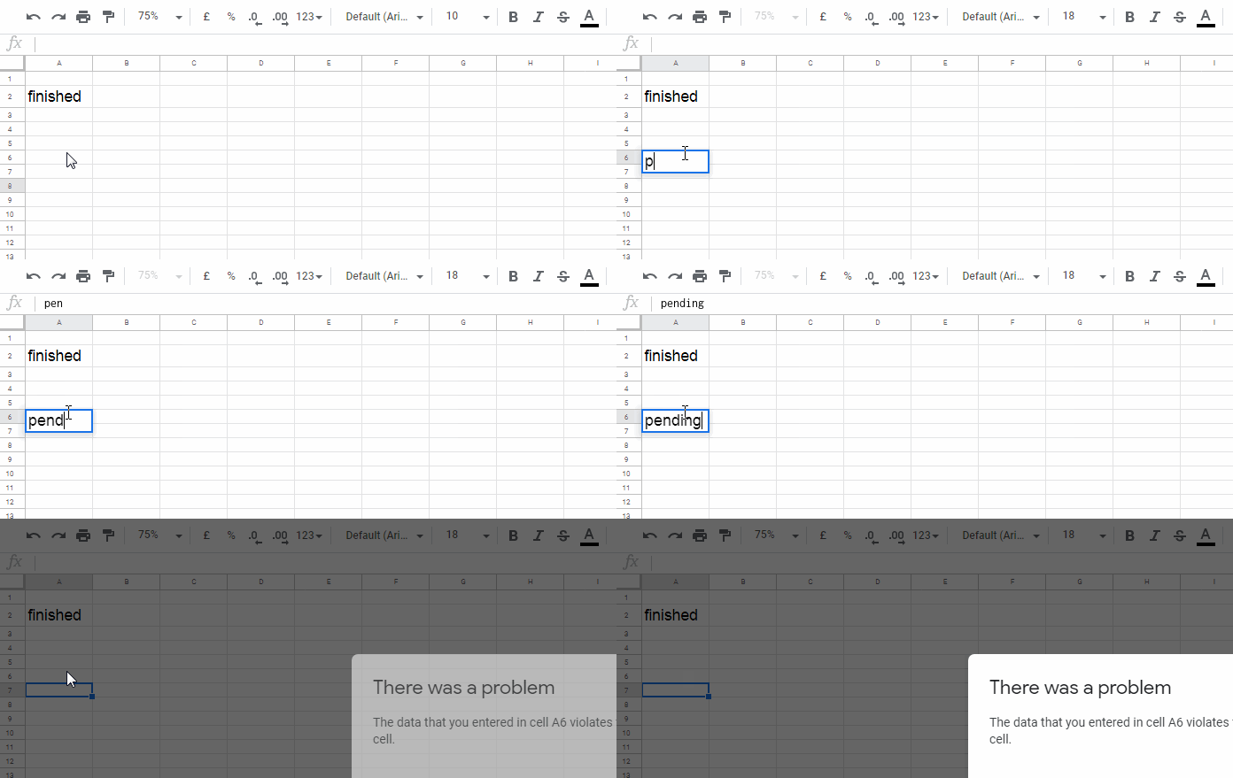
You can reject a list of items from being entered in a range using data validation in Google Sheets.
In this post, I’ll explain two helpful data validation tips:
- How to reject or restrict a list of specific items (such as item codes, item numbers, names, or any values) from being entered in a range.
- How to reject a list of items if those items are already present in another sheet or range.
Let’s go through these two types of data validation rules with examples.
How to Reject a List of Items Using Data Validation
Block (Reject Input of) a List of Values
Assume I want to reject entries like “pending”, “withheld”, or “amended” in column A. Here’s the formula to apply in data validation for that:
Formula #1:
=NOT(REGEXMATCH(TO_TEXT($A1), "(?i)pending|withheld|amended"))How to Use This Custom Formula in Data Validation
- Select the range you want to validate (e.g.,
A1:A). - Go to Data > Data validation.
- Under Criteria, select “Custom formula is”.
- Enter the formula above.
- Set the action to “Reject input”.
- (Optional) Add help text like: “You cannot enter ‘pending’, ‘withheld’, or ‘amended’.”
- Click Done.

This rule blocks input if it matches any of the listed values, regardless of case.
Note: If your data validation range starts from a different row (e.g.,
A10:Ainstead ofA1:A), make sure to update the formula reference from$A1to$A10to match the first cell in the range.
How the Formula Works
- REGEXMATCH checks if the cell contains one of the specified words.
- TO_TEXT converts any numeric input to text so that REGEXMATCH processes it.
- NOT flips the result: matching values become
FALSE, thus rejected.
Want to Reject Exact Matches Only?
Use this regular expression pattern instead of the one above:
(?i)^pending$|^withheld$|^amended$Can I Include Numbers?
Absolutely. The earlier REGEXMATCH formula works with numbers too—thanks to the TO_TEXT function.
However, if you’re applying the rule specifically in a numeric column, and want to block only specific numbers (like 1, 2.5, and 4.5), this approach is cleaner and more precise:
=ISNA(XMATCH($A1, HSTACK(1, 2.5, 4.5)))This returns TRUE (valid input) only when the entered number is not in the specified list.
How to Reject a List of Items from Another Sheet Using Data Validation
Let’s now address the same validation use case—but this time, the list of values to be rejected exists in another sheet (e.g., “Sheet2”).
We want to block entries in column A (Sheet1) if those entries match “pending”, “withheld”, or “amended” and if they already exist in a specified range in Sheet2.
Example Range Options
- A single cell:
Sheet2!$A$1 - A range:
Sheet2!$A$1:E$10 - Multiple rows:
Sheet2!$1:$1000(first 1000 rows)
Formula to Reject a List of Items in Column A if Present in Another Sheet
Formula #2:
=REGEXMATCH(TO_TEXT($A1),"pending|withheld|amended")*
ARRAYFORMULA(SUM(REGEXMATCH(TO_TEXT(Sheet2!$A$1:E$10), TO_TEXT($A1))*1))=0
To apply this formula, follow the same steps described earlier under “How to Use This Custom Formula in Data Validation.”
How This Formula Works
This formula has two parts:
Part 1 – Check for Blocked Terms
REGEXMATCH(TO_TEXT($A1),"pending|withheld|amended")Checks if the value entered in cell A1 matches any of the blocked terms (case-insensitive). Returns TRUE for a match.
Part 2 – Check if Value Exists in Another Sheet
ARRAYFORMULA(SUM(REGEXMATCH(TO_TEXT(Sheet2!$A$1:E$10), TO_TEXT($A1))*1))Searches the range Sheet2!A1:E10 to see if the same value already exists. If found, returns a number greater than 0.
Final Logic
= Part1 * Part2 = 0This condition allows the entry only if the value:
- Is not on the blocked list, or
- Is not present in
Sheet2!A1:E10
If both parts return TRUE, the formula evaluates to 1 * 1 = 1, which is FALSE, so the value is rejected.
Logic Scenarios
| Match in Blocked List | Match in Sheet2 | Result | Status |
|---|---|---|---|
| ✅ | ❌ | 1 * 0 = 0 | ✅ Allowed |
| ❌ | ✅ | 0 * 1 = 0 | ✅ Allowed |
| ✅ | ✅ | 1 * 1 = 1 | ❌ Blocked |
Want Exact Match in This Case Too?
Use the following tweaks:
- Update Part 1 with:
(?i)^pending$|^withheld$|^amended$- Update Part 2’s match pattern to:
"^" & $A1 & "$"So the complete updated formula becomes:
=REGEXMATCH(TO_TEXT($A1), "(?i)^pending$|^withheld$|^amended$") *
  ARRAYFORMULA(SUM(REGEXMATCH(TO_TEXT(Sheet2!$A$1:E$10), "^" & $A1 & "$") * 1)) = 0
Conclusion
That’s how you can reject a list of items in data validation in Google Sheets, whether using a hardcoded list or referencing values from another sheet. These methods help you control input efficiently and ensure cleaner data.
Resources
- How to Prevent Invalid Data Entry in Google Docs Spreadsheets
- How to Prevent Duplicates in Google Sheets
- The Best Data Validation Examples in Google Sheets
- Currency Formatting in Google Sheets Drop-Downs
- Restrict Entering Special Characters in Google Sheets (Data Validation)
- Restrict or Force Text Entry to All Caps, All Lower Cases, or Proper Case in Google Sheets


How can I restrict
&,$,%,#,@,!in just one formula in Google Sheets.Hi, Anu Bhatia,
Please see the “Resources” section at the bottom of this post.
There you can find the related tutorial. The title contains the term “special characters”.
Hello,
This is really useful thank you.
I am trying to do a similar thing with date times. I need to force the cell to be a date-time greater than the cell preceding it – are you able to help at all?
Hi, Alexander Markides,
=and(gt(B4,B3),isdate(B4),isdate(B3))This will only permit date-time in B4 if it’s greater than the date-time in B3.
You can use the same for a range.
For example, for the range B3:B10, the same formula should be applied for the data validation “cell range” B4:B10.