How to Query Non-Calendar Quarters in Google Sheets

Working with fiscal year data that doesn’t start in January? If you’re trying to group or summarize data by quarter in Google Sheets using the QUERY function, it can get tricky—especially when your fiscal year runs from April to March (or any non-calendar pattern). Since the QUERY function doesn’t natively recognize non-calendar quarters, you’ll need a small workaround to get it right.

In this post, I’ll walk you through how to adjust your dataset using formulas so you can easily query non-calendar quarters in Google Sheets—no scripts or manual editing required.

This tutorial is part of the Date Logic in QUERY hub.
Learn how date logic works in Google Sheets QUERY, including date criteria, month-based filtering, and DateTime handling.

Table of Contents

Sample Data

Our sample data tracks purchases of various products, including their quantity, rate, and amount.

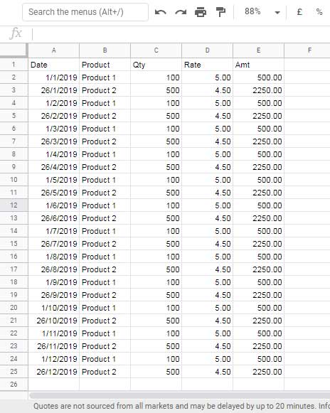
For this example, we assume the fiscal year runs from April to March, which means:

Q1 = Apr–Jun
Q2 = Jul–Sep
Q3 = Oct–Dec
Q4 = Jan–Mar (of the following calendar year)

Let’s see how to generate fiscal quarters and use them with the QUERY function.

👉 To follow along, feel free to copy this sample Google Sheet:

Copy Sample Sheet

Step 1: Create a Helper Column for Fiscal Quarters

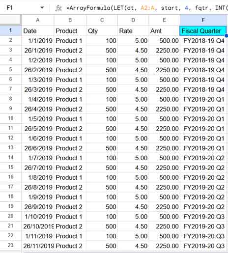
In the sample sheet, the date starts from cell A2. We’ll add a helper column in cell F1 (assuming columns A to E are occupied) to generate the fiscal quarter corresponding to each date.

Paste this formula in cell F1:

=ArrayFormula(LET(
   dt, A2:A, 
   start, 4, 
   fqtr, INT(MOD(MONTH(dt)-start, 12)/3+1), 
   fyrs, YEAR(dt)-(MONTH(dt)<start), 
   fyre, RIGHT(YEAR(dt)+(MONTH(dt)>=start), 2), 
   VSTACK("Fiscal Quarter", IF(dt="",," FY"&fyrs&IF(start=1,,"-"&fyre)&" Q"&fqtr))
))

This formula will return fiscal quarters like FY2019-20 Q1, FY2019-20 Q2, etc., based on an April–March fiscal year.

👉 If your fiscal year starts in a different month, just replace 4 (April) in the start variable with your fiscal year start month (e.g., 7 for July).

Screenshot of a helper column in Google Sheets showing fiscal quarter values like FY2019-20 Q1, generated using a custom formula for non-calendar year data

Formula Breakdown

start – The starting month of your fiscal year. In this example, 4 stands for April.
fqtr – Calculates the fiscal quarter based on the shifted start month.
fyrs – Derives the starting year of the fiscal year. If the month is before the fiscal start month, it uses the previous year.
fyre – Returns the last two digits of the ending year of the fiscal year (e.g., 20 for 2020).
VSTACK(...) – Combines the column header ("Fiscal Quarter") with the generated fiscal quarter values while skipping empty rows.

To learn more, check out this detailed guide:
Convert Dates to Fiscal Quarters & Years in Google Sheets

Step 2: Query Non-Calendar Quarters in Google Sheets

Now that we have fiscal quarters in column F, we can use the QUERY function to group and summarize data by quarter.

Query by Fiscal Quarter Only

To get the total amount per quarter:

=QUERY(A1:F, "SELECT F, SUM(E) WHERE F IS NOT NULL GROUP BY F LABEL SUM(E) 'Amount'", 1)

Result: Summary of Amounts by Fiscal Quarter

Fiscal Quarter	Amount
FY2018-19 Q4	8250
FY2019-20 Q1	8250
FY2019-20 Q2	8250
FY2019-20 Q3	8250
FY2019-20 Q4	2250

Explanation:

F refers to the Fiscal Quarter column.
E is the Amount column.
The formula groups by fiscal quarter and calculates the sum of amounts.

Query by Fiscal Quarter and Category

To break it down further by product:

=QUERY(A1:F, "SELECT F, B, SUM(E) WHERE F IS NOT NULL GROUP BY F, B LABEL SUM(E) 'Amount'", 1)

Result: Amounts Grouped by Fiscal Quarter and Product

Fiscal Quarter	Product	Amount
FY2018-19 Q4	Product 1	1500
FY2018-19 Q4	Product 2	6750
FY2019-20 Q1	Product 1	1500
FY2019-20 Q1	Product 2	6750
FY2019-20 Q2	Product 1	1500
FY2019-20 Q2	Product 2	6750
FY2019-20 Q3	Product 1	1500
FY2019-20 Q3	Product 2	6750
FY2019-20 Q4	Product 2	2250

Explanation:

This formula groups by both fiscal quarter and product.
Useful for comparing sales or performance across products per quarter.

Alternative: Use QUERY with Calendar Quarters

If your fiscal year follows the calendar year (i.e., starts in January), you don’t need a helper column. You can use the built-in QUARTER() and YEAR() scalar functions inside QUERY.

Without Category

=QUERY(A1:E, "SELECT QUARTER(A), YEAR(A), SUM(E) WHERE A IS NOT NULL GROUP BY QUARTER(A), YEAR(A) ORDER BY YEAR(A) LABEL SUM(E) 'Amount'", 1)

With Category

=QUERY(A1:E, "SELECT QUARTER(A), YEAR(A), B, SUM(E) WHERE A IS NOT NULL GROUP BY QUARTER(A), YEAR(A), B ORDER BY YEAR(A) LABEL SUM(E) 'Amount'", 1)

Note: When using QUARTER(), make sure to group by YEAR() and order by YEAR() to avoid mixing data from the same quarter across different years and to ensure correct sorting.

Conclusion

If you’re working with fiscal year data that doesn’t follow the January–December calendar, the default QUERY tools in Google Sheets fall short. But with a simple helper formula, you can generate fiscal quarters and then query non-calendar quarters in Google Sheets just like calendar-based data.

This approach works great for reporting, financial analysis, and dashboards—without any manual editing or Apps Script.