The MOD function is a mathematical function in Google Sheets that returns the remainder after a division operation. It is important not to confuse it with the MODE function, which is used in statistics to find the most frequently occurring number in a dataset.
Purpose of the MOD Function
The MOD function is useful in various scenarios where you need to determine remainders from divisions, especially in conditional formatting, filtering, or creating complex formulas.
Syntax
MOD(dividend, divisor)- dividend: The number you want to divide to find the remainder.
- divisor: The number by which you want to divide the dividend. Note that the divisor cannot be zero, as this will result in an error.
Examples of Using the MOD Function in Google Sheets
Here are a few examples to help you understand how to use the MOD function:
- Example 1: Simple Division
- Formula:
=MOD(6, 4) - Result: 2
- Explanation: When 6 is divided by 4, the remainder is 2.
- Formula:
- Example 2: Division with No Remainder
- Formula:
=MOD(9, 3) - Result: 0
- Explanation: 9 divided by 3 has no remainder.
- Formula:
- Example 3: Divisor is Zero
- Formula:
=MOD(5, 0) - Result:
#DIV/0!Error - Explanation: Division by zero is undefined, resulting in an error.
- Formula:
- Example 4: Negative Divisor
- Formula:
=MOD(10, -3) - Result: -2
- Explanation: The remainder of 10 divided by -3 is -2.
- Formula:
- Example 5: Timestamp
- Formula:
=MOD("2024-01-01 10:10", 1) - Result: 0.4236111111 (When formatted as time, this result will display as 10:10 AM)
- Formula:
Real-Life Applications of the MOD Function
The MOD function can be quite useful in various real-life scenarios. Here are a few applications:
- Identifying Even or Odd Numbers: You can use MOD to check whether a number is even or odd. For example,
=MOD(A1, 2)returns 0 for even numbers and 1 for odd numbers. - Cycle Through Lists: MOD can be used to cycle through a list at regular intervals. For instance, if you want to get every third item from a list, you can use the formula
=FILTER(B1:B10, MOD(SEQUENCE(10), 3) = 1). This formula generates a sequence from 1 to 10 and uses MOD to filter the items in the range B1:B10 based on the condition that the row number is congruent to 1 when divided by 3. This approach is useful for extracting data at specific intervals, such as sampling every third entry.
Combining the MOD Function with Other Functions
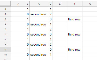
Some functions in Google Sheets accept other functions as arguments, and MOD is no exception. Here’s an example of how you can use MOD in combination with other functions to create more complex formulas.
- Formula in Cell B1:
=ARRAYFORMULA(MOD(ROW(A1:A10), 2)) - Formula in Cell D1:
=ARRAYFORMULA(MOD(ROW(A1:A10), 3))

Both of these formulas return an array of values based on the row numbers. The first formula returns 0 for even rows and 1 for odd rows, while the second formula returns 0 for every third row.
You can use these results to filter or extract data from your spreadsheet. For example, you can use the FILTER function to get all values in every second or third row.
We have already seen a similar example with the SEQUENCE and FILTER combo earlier in this tutorial.
Conclusion
The MOD function in Google Sheets is a powerful tool for performing mathematical operations and creating complex formulas. Whether you’re checking for even numbers, cycling through lists, or filtering data, understanding how to use MOD effectively can enhance your spreadsheet skills.
We hope you find this tutorial useful! Enjoy exploring the possibilities with the MOD function!


I use MOD with other functions to quickly sum up columns of time durations and convert them into an
h:mmformat.=CONCATENATE(TRUNC(90/60),":",MOD(90,60))Or as a quick validation when numbers have to divide evenly.
=if(MOD(4,2)=0,"pass","fail")Both of these are mainly useful when dealing with multiple cells in large sheets. For a single cell, I just use a calculator.