


We can match available and required items in rows or columns and highlight if all of them are available in Google Sheets.
Imagine you are a pharmacist. A customer/patient only wants to buy medicines from you if all the items in the prescription are available with you.
If unavailable, he wishes to check it with another pharmacist.
If you have maintained the stock in Google Sheets, you can use conditional formatting to identify if all the required items are available.
When all the medicines in the prescription match within the available stock, then highlight that entire record. Otherwise, highlight only the nonavailable item(s) in red.
How to match available and required items and highlight if all of them are available in Google Sheets?
Of course, there is no built-in rule for this in Google Sheets Conditional formatting.
You must write a custom formula based on the orientation of your data.
We will start with horizontally arranged data first.
Match Available and Required Items (Ingredients) and Highlight Entire Row
In the following table, I have the name of a few ingredients in row # 1.
I have checked (tick marked) the available ingredients in row # 2 using the menu Insert > Tick box.
There are two recipes, “Cauliflower Cheese” and “Paneer Masala Fry,” in rows 3 and 4, respectively. You can add as many recipes as you want.
The “ok” in these rows mark the required ingredients to prepare these recipes.
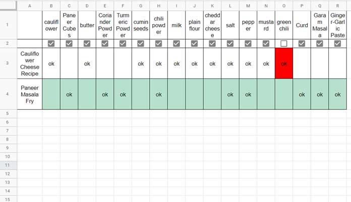
As per the above highlighting, I can prepare “Paneer Masala Fry” as all the ingredients are available for this recipe.
Regarding “Cauliflower Cheese Recipe,” one of the ingredients, i.e., “green chili,” is not available.
To match the available and required items (ingredients) and then highlight the entire row, we can use the below rule for the range B3:R100.
Rule_1:
=and($A3<>"",countif(ArrayFormula($B$2:$R$2&$B3:$R3),"FALSEok")=0)For the first recipe, “green chili” is out of stock. So the formula didn’t highlight B3:R3.
The following rule for B3:R100 highlights the non-available item (ingredient).
Rule _2:
=and(len($A3),B$2=FALSE)To insert the above two rules to match available and required items and conditionally highlight, please follow the below 6+ steps.
- Select B3:R100.
- Format > Conditional formatting (menu options).
- Make sure that the active “Conditional format rules” tab is “Single color” (the default tab).
- Select Format rules > Custom formula is.
- Copy-paste Rule_1.
- Click “Done.”
- Click “Add another rule” to insert Rule_2. This time, choose a different color, preferably red, to highlight the non-available value/item/ingredient.
Formulas (Highlight Rules) Explanation
There are two rules, and rule_2 is pretty simple. So let me start from that.
Rule_2 Explanation
It highlights non-available items (ingredients).
In this, =and(len($A3),B$2=FALSE), the bold part tests whether the tick box is unchecked (FALSE) in B2:R2 and highlights the ‘entire column’.
And the ‘entire’ column may affect by the following.
- The
len($A3(first part) checks A3:A100. It ensures that the rule won’t highlight blank rows. - The conditional format gives priority to the first rule (Rule_1). If it highlights an entire row, the highlighting of Rule_2 won’t be visible.
Rule_1 Explanation
It matches available and required items and highlights if all the required items are available.
The bold part combines B2:R2 (availability) with B3:R3, B4:R4, B5:R5, and so on (requirements) in each row.
Here is what happens with the first recipe.
=and($A3<>"",countif(ArrayFormula($B$2:$R$2&$B3:$R3),"FALSEok")=0) 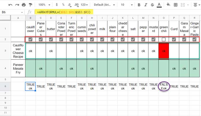
If any cell has the value “FALSEok”, that means the item (here the ingredient) is not available (FALSE) but is required (ok) for the recipe.
If the COUNTIF on this array result returns 0 (zero), that means there is no “FALSEok.” So the formula highlights that row.
In the formula, $B$2:$R$2 is absolute (fixed), and in $B3:$R3, the row is relative.
Match Available and Required Items (Ingredients) and Highlight Entire Column
Below, I am changing the orientation of the above data from horizontal to vertical. So, we must modify the formula rules.
But please note that I suggest horizontal data for matching available and required items and highlighting in Google Sheets. That seems more reader-friendly.
But some of you may prefer column-wise (vertical) data. Here you go!
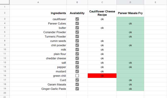
Yep! Once again, I am considering the same data (recipes and ingredients). Here are the conditional format rules.
Rule_1: =and(C$2<>"",Countif(ArrayFormula($B$3:$B$19&C$3:C$19),"FALSEok")=0)
Rule_2: =and(len(C$2),$B3=FALSE)
The “Apply to range” of both of these rules is C3:19.
I have modified the formulas to match the orientation of the data. There are no other changes. So I am not explaining the logic again.
That’s all. Thanks for the stay. Enjoy!