Get Last Saturday of Any Given Month and Year in Google Sheets

Published on

When preparing financial statements, you may want to find the last Saturday of any given month and year in Google Sheets.

It may be because your company ends its fiscal year on the same day of the last week, here Saturday, of a month every year.

If you use Google Sheets, please note there is no specific function to meet that requirement.

You may require to write a formula using multiple functions.

Here I am using the combination of WEEKDAY and EOMONTH date functions for that.

Pre-Requisites – Input Date Values and Formatting

Assume you want to use a formula to get the last Saturday of a given month, i.e., September 2021, in Google Sheets.

You can input the values for the formula in either of the below two ways.

  1. Enter the text “September” (without double quotes) in cell A2 and 2021 in cell B2.
  2. 01/09/2021 (or any date that falls in September 2021) in cell C2 (you feel free to format it to just (MMM) using Format > Number > Custom number format).

If you follow option 1, you may additionally be required to use the following formula in cell C2.

=date(B2,month(A2&1),1)

The highlighted formula converts the month name in text to the month number.

Here I am following option 2. So, in cell C2, enter any date that falls in that month and year, for example, 01/09/2021 (DD/MM/YY).

My formula in cell D2 will return the date 25/09/2021, i.e., the last Saturday of that given month and year in cell C2.

Formula to Get the Last Saturday of Any Given Month in Google Sheets

I guess you have already entered the above input value(s) in the given cell(s). If so, in cell D2, insert the following combination formula, and voila!

=eomonth(C2,0)-(WEEKDAY(eomonth(C2,0))<>7)*weekday(eomonth(C2,0))

If you input 01/01/2022 in cell C2, you will get 29/01/2022 in cell D2.

We can use an array formula to get the last or final Saturday in the given month in the subsequent years.

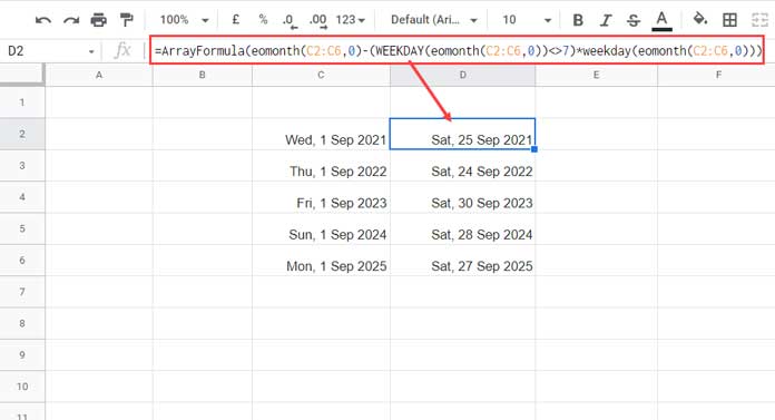
For example, if the end month of the fiscal year is September, the company’s year-end could fall on any date from September 24 to September 30 in the years 2021-2025.

E.g.:-

Enter 01/09/2021, 01/09/2022, 01/09/2023, 01/09/2024, and 01/09/2025 in cell range C2:C6.

Insert the below array formula in cell D2 which we get after modifying C2 in the non-array formula to C2:C6 and wrapping it with the ArrayFormula function.

=ArrayFormula(eomonth(C2:C6,0)-(WEEKDAY(eomonth(C2:C6,0))<>7)*weekday(eomonth(C2:C6,0)))
Last Saturday in Every September

To get the last Saturday in all the months in a given year in Google Sheets, feed the following dates in the array C2:C13.

=ArrayFormula(eomonth(C2:C13,0)-(WEEKDAY(eomonth(C2:C13,0))<>7)*weekday(eomonth(C2:C13,0)))
Last Saturday in All Months in an Year

The formula is the same except for the cell range/array.

Formula Explanation

There are two parts in the formula that returns the last Saturday of any given month in Google Sheets.

Please note that I’m explaining the above non-array formula.

Generic Formula: part_1 - part_2_a*part_2_b

Part_1:

eomonth(C2,0)

It converts the given date in cell C2 to the end of the month date.

Part_2:

(WEEKDAY(eomonth(C2,0))<>7)*weekday(eomonth(C2,0))

Let’s further bifurcate it into part_2_a and part_2_b.

Part_2_a:

(WEEKDAY(eomonth(C2,0))<>7)

The part_2_a returns TRUE (1) if the weekday of the end of the month of the date in cell C2 is not equal to 7 (Saturday) else FALSE (0).

Part_2_b:

weekday(eomonth(C2,0))

The part_2_b will return the weekday of the month of the date in C2.

In essence, the part_2 will be;

  • If the weekday of the end of the month C2 is not Saturday, 1*weekday_of_eomonth_of_C2.
  • If the weekday of the end of the month C2 is Saturday, 0*weekday_of_eomonth_of_C2.

We are just subtracting this output from part_1 to get the last Saturday of the given month.

That’s all about finding the final or last Saturday of any given month and year in Google Sheets.

Thanks for the stay. Enjoy!

Prashanth KV
Prashanth KV
Your Trusted Google Sheets and Excel Guide Prashanth KV brings a wealth of experience in Google Sheets and Excel, cultivated through years of work with multinational corporations in Mumbai and Dubai. As a recognized Google Product Expert in Docs Editors, Prashanth shares his expertise through insightful blogging since 2012. Explore his blog for practical tips and guidance on maximizing your spreadsheet skills.

Lookup Previous Values Dynamically in Excel and Google Sheets

Sometimes, you may want to look up the previous values relative to the current...

Sort Data but Keep Blank Rows in Excel and Google Sheets

Using a dynamic array formula or the FILTER command, we can sort data and...

Lookup Values Under Categories in Excel and Google Sheets

We can use a combination of XLOOKUP and VLOOKUP in both Excel and Google...

Extract Items Under a Category from the Same Column in Excel

In Excel, you can use a combination of the XLOOKUP and DROP functions to...

More like this

XMATCH Row by Row: Finding Values Across a Range in Google Sheets

Using the BYROW function with XMATCH in Google Sheets allows us to match values...

Limit Formula Expansion to a Specific Row in Google Sheets

In this tutorial, I’ll explain how to limit the expansion of an array formula...

3-D Referencing Structured Data Tables in Google Sheets

When you have several tables within a single sheet—not across multiple sheets in a...

LEAVE A REPLY

Please enter your comment!
Please enter your name here

This site uses Akismet to reduce spam. Learn how your comment data is processed.