There are four main ways to join text in Google Sheets: using JOIN, TEXTJOIN, CONCATENATE, and ampersand (&) functions.

The CONCAT and QUERY functions can also be used to join text, but they are not as popular as the other four functions.

The CONCAT function is a simpler function that does not offer as many options as the JOIN or TEXTJOIN functions.

The QUERY function is a more powerful function that can be used to manipulate data in Google Sheets. It is not specifically designed for joining text, but it can do so by specifying an arbitrarily large number in the QUERY header. We will see how to do this in another tutorial.

I have already explained the use of CONCATENATE and the ampersand. Now let us learn the functions JOIN and TEXTJOIN. I think it is important to know the difference between these three functions so that you can choose the right one for your needs.

How to Use JOIN Function in Google Sheets

The JOIN function in Google Sheets joins the elements of one or more one-dimensional arrays, where the joined elements can be separated by a given delimiter.

Syntax:

JOIN(delimiter, value_or_array1, [value_or_array2, …])

• delimiter: The character or string to place between each joined value. This can be a comma, space, hyphen, or any other value.
• value_or_array1: The value or values to be joined. This can be a single cell, a range of cells (one-dimensional), or a list of values.
• value_or_array2, …: Additional values or arrays (one-dimensional) to be joined.

JOIN Formula Example 1:

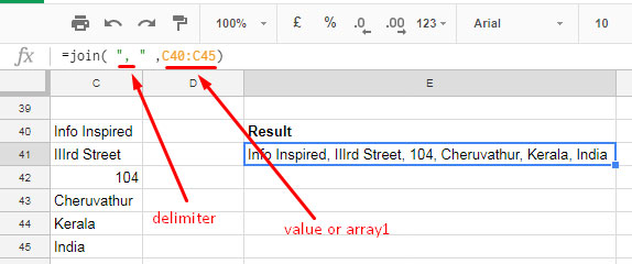
=JOIN(", ",C40:C45)

The above JOIN formula joins the values (addresses in separate rows) in the cell range C40:C45. When joining, the formula places a comma and space as delimiters to return a proper address in a single cell.

JOIN Formula Example 2:

=JOIN(": ",C40:C42,D40:D42)

In this Google Sheets JOIN function example, you can see that there are two arrays in use. It returns the same result as example 1 above, with the only difference being the delimiter in use. In this case, the delimiter is a colon (;) and a space, instead of a comma (,) and a space.

The below formula will not work as the JOIN function only supports one-dimensional arrays.

=join( " : " ,C40:D42)

Here is the use of the Google Sheets TEXTJOIN function.

How to Use TEXTJOIN Function in Google Sheets

Google Sheets TEXTJOIN function joins text from multiple arrays where the joined texts can be separated by a given delimiter.

Syntax:

TEXTJOIN(delimiter, ignore_empty, text1, [text2, …])

• delimiter: The character or string to place between the joined texts. This can be a comma, space, hyphen, or any other value.
• ignore_empty: A Boolean TRUE or FALSE (you can also use 1 or 0 [zero]). It controls blank cells in the selected range.
• text1: The array containing the text to join or the text itself. This can be a single cell, a range of cells, or a list of values.
• text2, …: To include additional arrays (usually to combine distant ranges) or texts.

Here I will try to explain the syntax with a few examples.

The TEXTJOIN Formula Example 1:

=TEXTJOIN(", ",TRUE,C52:D53)

Please note that there are no blank cells in the selected range. Therefore, the result will be the same whether you use FALSE or TRUE for the ignore_empty argument.

The TEXTJOIN Formula Example 2:

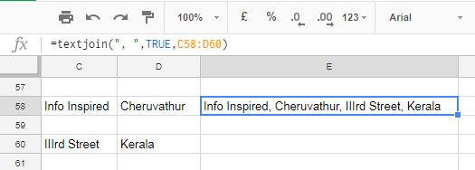
=TEXTJOIN(", ",TRUE,C58:D60)

Here, there are blank cells in between the selected array. Therefore, I used a Boolean TRUE in the formula to ignore these blank cells.

The TEXTJOIN Formula Example 3:

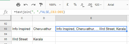
See what happens when the ignore_empty argument is set to FALSE in the formula when there are blank cells. The comma delimiter separator will also appear for the blank cells.

=TEXTJOIN(", ",FALSE,C63:D65)

Note: When using a two-dimensional array in the TEXTJOIN function, the formula combines the values by row, not by column.

Comparison of Google Sheets JOIN, TEXTJOIN, and CONCATENATE Functions

I am using three text join functions—JOIN, TEXTJOIN, and CONCATENATE—and the fourth one, &, to join the texts in A1:G1 below. See how each formula differs.

My expected result is as follows: JOIN✓ ME✓ PLEASE✓ WITH✓ A✓ TICK MARK

1. Using the AMPERSAND (&):

=A1&"✓ "&B1&"✓ "&C1&"✓ "&D1&"✓ "&E1&"✓ "&G1

2. Using the CONCATENATE Text Function:

=CONCATENATE(A1,"✓ ",B1,"✓ ",C1,"✓ ",D1,"✓ ",E1,"✓ ",G1)

3. Using the JOIN Text Function:

=JOIN("✓ ",A1:E1,G1)

4. Using the TEXTJOIN Text Function:

=TEXTJOIN("✓ ",TRUE,A1:G1)

I know you want to learn how to use the QUERY function to combine values in Google Sheets. Please check out this tutorial: The Flexible Array Formula to Join Columns in Google Sheets.