How to Use ISNONTEXT Function in Google Sheets [Practical Use]

The ISNONTEXT is an info type function and not common in use in Google Sheets. But it has some real use that many users didn’t explore so far. In this new tutorial, learn how to use ISNONTEXT function in Google Sheets.

The function ISNONTEXT simply checks whether a value is non-textual. If the value referred in this formula is not text, it returns TRUE, else FALSE.

It’s very useful in logical tests and also in the Query function in Google Sheets! You can learn these tips along with the use of the ISNONTEXT function in Google Sheets.

Earlier I’ve posted a tutorial related to the use of the Google Sheets function N, which is a ‘lifesaver’. You can include ISNONTEXT in the same category.

How to Use ISNONTEXT Function in Google Sheets

Syntax:

ISNONTEXT(value)

I don’t think there is anything specific to mention about the arguments in this function. So let’s move to examples.

ISNONTEXT Formula 1

=ISNONTEXT("infoinspired")

ISNONTEXT Formula 2

=ISNONTEXT(105)

In the above two formulas, the first one returns the Boolean FALSE and the second formula returns the Boolean TRUE.

Practical Use of Google Sheets ISNONTEXT Formula

At the beginning of this Google Sheets tutorial, I’ve mentioned you about the use of ISNONTEXT in IF logical test and Query.

See that two unexplored use of this function below.

1. ISNONTEXT in IF Logical Test

Example Dataset:

ISNONTEXT in IF Logical Test

If you are familiar with spreadsheet applications you can understand one thing. In the above sample dataset, column F is left blank. There I want to find the product in each row.

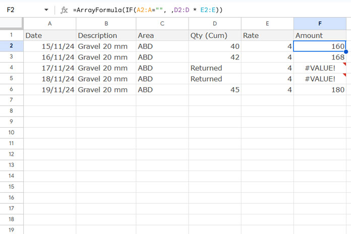
=ArrayFormula(D2:D8*E2:E8)

The above array formula can do the multiplications. You should apply this formula in F2. It expands the results.

The formula would return two #VALUE! errors that in the Cells F4 and F7 because of the text values in corresponding rows in Column D.

ISNONTEXT to replace errors with corresponding row values

You can easily remove these errors by wrapping the above formula with an IFERROR function.

=iferror(ArrayFormula(D2:D8*E2:E8))

The above formula would remove the errors and leave those cells blank. Instead of replacing the errors with blank cells, you can put any value, possibly zero or any custom message.

This formula replaces the errors with the value 0.

=iferror(ArrayFormula(D2:D8*E2:E8),0)

Now please again check the cells D4 and D7 which contains the string “Nil” and “Yet to update” respectively.

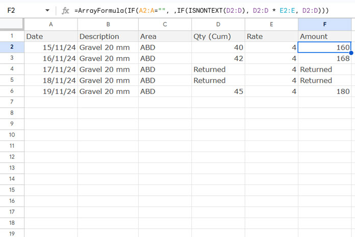
I want those strings in F4 and F7. Here comes the use of the said ISNONTEXT function in Google Sheets.

=ArrayFormula(if(isnontext(D2:D8),D2:D8*E2:E8,D2:D8))

The output would be as follows.

ISNONTEXT formula example

2. The Use of the Function ISNONTEXT in Google Sheets Query

Mixed content columns are always an issue in the Query function. In the above example Column D is an example of the mixed data type.

Similar: Google Sheets Query to Filter Numbers Only From Mixed Data Column

In such cases the minority data types, here in column D it’s string, are considered as null values. So the result may or may not be perfect.

To solve this ‘problem’ normally Google Sheets users use the To_Text function which converts the entire column values to text.

It’s not ideal in all situations. But it’s the best when you want to filter out blank rows in Query.

Must Read: How to Use To_text Function in Google Sheets [Also the Use in Query]

When you convert date or numbers to text, using them in calculations will be almost difficult. So we can use Google Sheets ISNONTEXT function as an alternative solution to To_Text.

Let me explain with one example how to use ISNONTEXT Function in Google Sheets Query.

=query({A2:E8})

See how the above data range replaced in the below formula with the help of the ISNONTEXT function.

=ArrayFormula(query({A2:C8,if(ISNONTEXT(D2:D8),D2:D8,0),E2:F8}))

This formula replaces the string in the mixed content column D with the value 0.

You can tweak this formula a little bit to filter out numbers in the column and retain the string. See that formula.

=ArrayFormula(query({A2:C8,if(ISNONTEXT(D2:D8),"-",D2:D8),E2:F8}))

Here the formula replaces the numbers with the character “-” in Column D.

The above two variations of ISNONTEXT can be replaced by simpler functions like the N or T. That’s all. Enjoy!

Prashanth KV
Prashanth KV
Your Trusted Google Sheets and Excel Guide Prashanth KV brings a wealth of experience in Google Sheets and Excel, cultivated through years of work with multinational corporations in Mumbai and Dubai. As a recognized Google Product Expert in Docs Editors, Prashanth shares his expertise through insightful blogging since 2012. Explore his blog for practical tips and guidance on maximizing your spreadsheet skills.

Lookup Values Under Categories in Excel and Google Sheets

We can use a combination of XLOOKUP and VLOOKUP in both Excel and Google...

Extract Items Under a Category from the Same Column in Excel

In Excel, you can use a combination of the XLOOKUP and DROP functions to...

How to Create a Searchable Table in Excel Using the FILTER Function

Finding specific records, or rows containing the required information, is straightforward in Excel using...

Time Sequences in Excel by Minute, Hour, or Second Increments

Creating time sequences, whether by hour, minute, or second increments in Excel, can be...

More like this

XMATCH Row by Row: Finding Values Across a Range in Google Sheets

Using the BYROW function with XMATCH in Google Sheets allows us to match values...

Limit Formula Expansion to a Specific Row in Google Sheets

In this tutorial, I’ll explain how to limit the expansion of an array formula...

3-D Referencing Structured Data Tables in Google Sheets

When you have several tables within a single sheet—not across multiple sheets in a...

LEAVE A REPLY

Please enter your comment!
Please enter your name here

This site uses Akismet to reduce spam. Learn how your comment data is processed.