This tutorial explains how to use the ISBETWEEN function in Google Sheets.

Purpose: We can use this function to check whether a value (or values) falls between two other values and return TRUE or FALSE based on the result.

Before this function was introduced, we relied on comparison operators like >, >=, <, and <=, or corresponding operator functions. In most cases, we also had to use the AND logical operator. Writing array formulas (single formulas for multiple rows) using those methods was somewhat complex.

The ISBETWEEN function in Google Sheets simplifies this process. I’ll walk you through the usage with examples. But first, let’s take a look at the function syntax.

ISBETWEEN Function in Google Sheets – Syntax and Arguments

Syntax:

ISBETWEEN(value_to_compare, lower_value, upper_value, [lower_value_is_inclusive], [upper_value_is_inclusive])

Arguments:

There are five arguments in ISBETWEEN, with the last two being optional.

All the arguments are pretty self-explanatory.

The two optional arguments accept TRUE or FALSE. If set to TRUE, the respective lower or upper value is inclusive. If set to FALSE, they are exclusive.

By default, both optional arguments are set to TRUE. So, include them only when you want to exclude one or both limits.

Examples to Use ISBETWEEN Function in Google Sheets

You can use ISBETWEEN with numbers, dates, or even letters.

Numeric Value in value_to_compare

Assume cell B2 contains the value 50. You want to test if it’s between 25 and 75 (inclusive):

=ISBETWEEN(B2, 25, 75)

No need to specify the optional parameters, as both limits are inclusive by default.

Earlier Workarounds:

Before we had the ISBETWEEN function, we used:

=AND(B2>=25, B2<=75)

or:

=(B2>=25)*(B2<=75) // returns 1 for TRUE and 0 for FALSE

The second method supports array formulas (e.g., B2:B instead of B2). More on that later.

Now back to ISBETWEEN.

If cell B3 contains 25, then:

=ISBETWEEN(B3, 25, 75) → TRUE  
=ISBETWEEN(B3, 25, 75, FALSE, FALSE) → FALSE

The second formula returns FALSE because both ends are exclusive.

Date in value_to_compare

Assume cell A2 contains the date 16-Mar-2021.

To check if it falls between 1-Jan-2021 and 31-Mar-2021 (inclusive):

=ISBETWEEN(A2, DATE(2021, 1, 1), DATE(2021, 3, 31))

⚠️ Make sure the lower_value and upper_value are specified using the DATE function to avoid formatting issues.

Letter (Alphabet) in value_to_compare

Let’s say you want to test if the letters in B1:B26 are between "F" and "L".

In cell C1, enter:

=ISBETWEEN(B1, "F", "L")

Then drag down.

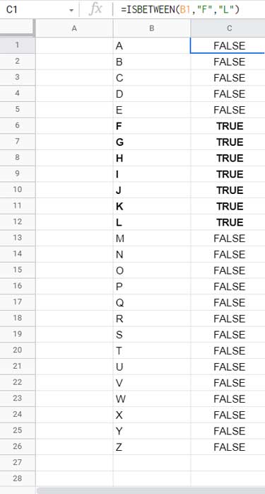
Note: This formula is case-insensitive, meaning it treats "l" and "L" the same.

ISBETWEEN Array Formula Use

One major advantage of the ISBETWEEN function in Google Sheets is that it accepts arrays or ranges in value_to_compare.

Instead of copying the formula down, simply use:

=ISBETWEEN(B1:B26, "F", "L")

✅ It auto-expands like Excel’s dynamic arrays—no need for ARRAYFORMULA.

Alternative:

=ArrayFormula((B1:B26 >= "F") * (B1:B26 <= "L"))

This returns 1 for TRUE, 0 for FALSE.

IF with ISBETWEEN Function in Google Sheets

Often, combining ISBETWEEN with the IF function is more practical.

Example:

Members must submit a form on or before 10-Mar-2021. If submitted after, return "Reject".

Assume the submission date is in cell A2:

=ISBETWEEN(A2, 0, DATE(2021, 3, 10))

To return "Reject" if outside the range:

=IF(ISBETWEEN(A2, 0, DATE(2021, 3, 10)), , "Reject")

Conclusion

If your formula returns #NUM!, check that lower_value and upper_value are of the same type.

For example:

✅ Correct: 1, 100
❌ Incorrect: "1", 100

Before wrapping up, one more note: this function has changed significantly since its launch. Initially, it required ARRAYFORMULA for range expansion. Also, ranges were previously allowed in lower_value and upper_value, which no longer works the same way.

That’s all. Thanks for the stay. Enjoy!

Resources

• ISBETWEEN Function in Conditional Formatting in Google Sheets
• How to Use ISBETWEEN with Filter Formula in Google Sheets
• COUNTIFS with ISBETWEEN in Google Sheets