With the IMPORTDATA function in Google Sheets, you can easily import a Comma-Separated Values (CSV) file into Google Sheets in a tabular format. The IMPORTDATA function also supports importing Tab-Separated Values (TSV) files.
CSV and TSV files are simple text formats that store and exchange tabular data between applications. What are the differences between these formats, and how are they used?
- CSV: The values are separated by commas.
- TSV: The values are separated by tab characters.
These formats allow data to be exchanged between systems that support such file formats. Google Sheets supports both formats, and the IMPORTDATA function is one method for bringing this data into Sheets while maintaining the tabular structure.
In some cases, the imported data may not retain its tabular form. If this happens, you can use functions like QUERY or SPLIT to properly adjust and format the imported data.
IMPORTDATA Function in Google Sheets – Formula Examples
Syntax of the IMPORTDATA Function:
IMPORTDATA(url)Example Formula:
Google provides thorough documentation on the IMPORTDATA function, and I’ll demonstrate a similar example here. Additionally, I’ll show how to limit the imported data to specific rows, columns, or even a single cell.
In this example, we’ll import a CSV file containing population estimates from the U.S. Census Bureau’s website. This data comes from their population estimates program for U.S. cities and towns between 2020 and 2023.
To use the IMPORTDATA function:
- Open a new Google Sheets file.
- In cell A1, enter the following formula:
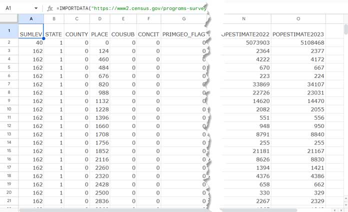
=IMPORTDATA("https://www2.census.gov/programs-surveys/popest/datasets/2020-2023/cities/totals/sub-est2023_1.csv")This formula will import the population estimate data in a tabular format.

Apply Data Manipulation Techniques to Imported Data
You can manipulate the imported data using the QUERY function to filter or limit the rows and columns returned.
Limit Rows Using QUERY with IMPORTDATA
You can limit the number of rows imported with a QUERY formula like this:
=QUERY(IMPORTDATA("https://www2.census.gov/programs-surveys/popest/datasets/2020-2023/cities/totals/sub-est2023_1.csv"), "SELECT * LIMIT 10")This formula limits the output to the first ten rows of the imported data. You can adjust the number to return more or fewer rows as needed.
Limit Columns Using QUERY with IMPORTDATA
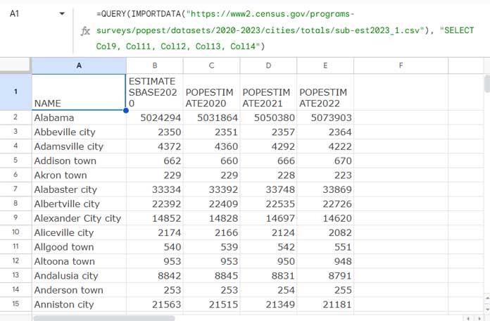
The default dataset contains 15 columns, but many of them might be irrelevant. You can limit the columns using the following formula:
=QUERY(IMPORTDATA("https://www2.census.gov/programs-surveys/popest/datasets/2020-2023/cities/totals/sub-est2023_1.csv"), "SELECT Col9, Col11, Col12, Col13, Col14")This formula returns only columns 9 and 11 to 14 from the dataset.

You can replace these column references with others based on your requirements.
Use Conditions with IMPORTDATA
While the IMPORTDATA function itself doesn’t support conditions, you can combine it with the QUERY function to filter data based on specific conditions.
For example, to import only the data for Allgood town:
=QUERY(IMPORTDATA("https://www2.census.gov/programs-surveys/popest/datasets/2020-2023/cities/totals/sub-est2023_1.csv"), "SELECT Col9, Col11, Col12, Col13, Col14 WHERE Col9='Allgood town' ")This formula imports only the rows where column 9 equals “Allgood town” and selects the specified columns.
Importing TXT Files Using the IMPORTDATA Function
In addition to CSV and TSV, you can also import text (TXT) files with the IMPORTDATA function in Google Sheets. However, the output may not always be in a tabular form.
To format the imported text into a table, you can use the SPLIT function. Here’s a generic formula:
=ARRAYFORMULA(SPLIT(QUERY(IMPORTDATA("your_text_file_URL"), "SELECT * OFFSET 5", 0), " "))In this formula:
- Replace “your_text_file_URL” with the actual URL of the TXT file.
- Adjust the OFFSET value (currently 5) to skip the appropriate number of rows if needed.
Alternatively, if the text file uses a consistent delimiter (like a comma), a simpler version can work:
=ARRAYFORMULA(IFERROR(SPLIT(IMPORTDATA("text_file_URL"), ",")))In this version, the system splits the data by commas. If your file uses a different delimiter, like a semicolon, replace the comma in the formula with the correct delimiter.
Conclusion
The IMPORTDATA function in Google Sheets is a powerful tool for importing external data in CSV or TSV formats while maintaining a tabular structure. If your imported data isn’t formatted correctly, you can use additional functions like QUERY and SPLIT to manipulate and adjust the data.
If you have any questions about using the IMPORTDATA function in Google Sheets, feel free to ask!


I tried your last example, where my “csv” file is delimited with a pipe.
There’s a problem with rows of data that don’t have any data between the pipes, it eliminates them from the results for some reason, putting data in the wrong columns.
What’s causing this?
Query:
=ArrayFormula(IFERROR(split(IMPORTDATA("url_to_csv_data"),"|")))Hi, Paul,
If possible, please share a sample of your data. You can share the URL below which won’t be published.
Can you do a query to ignore certain columns? Like
"Select * except(col2,col7)"Hi, Ivan,
Nope! Instead, you can include the required columns like
"Select Col1, Col2, Col3, Col6". I know it’s a difficult task to include so many columns likewise.The good thing is that you can do it dynamically.
How to Get Dynamic Column Reference in Google Sheets Query.
Hi Prashanth
Thanks for your answer.
Here is the url with the Sheet.
– link (Sheets) removed by the admin –
Hi, PETIT,
Wrap the cell reference with the T function.
=importdata(t(D8))Best,
Hello! I need some help with importdata function. Can you please help me?
Here is my formula (not finished)
={IMPORTDATA(D4); IMPORTDATA(D5); IMPORTDATA(D6); IMPORTDATA(D7); IMPORTDATA(D8); IMPORTDATA(D9); IMPORTDATA(D10); IMPORTDATA(D11); IMPORTDATA(D12); IMPORTDATA(D13)}(i need it to go to D978)
First question: do you know a way not to make it manually? (maybe the easiest question)
Second question: cells from D4 to D978 are, in fact, dates as 2019-08-27
I need the dates written in the first (for example) column for every CSV I import.
Is this possible with a simple formula? Thanks for your help and your daily blog.
Hi, Petit,
Can you share a demo sheet or screenshot link?
To capture your Google Sheets screenshot and get the link you can depend on online screenshot tool like “Lightshot”. Here is the link to that site: https://prnt.sc/
Best,