This post explains how to use the IMPORTFEED function to keep track of updates to your favorite websites in Google Sheets.
The IMPORTFEED function helps you import an RSS (Really Simple Syndication) or Atom feed into Google Sheets.
RSS and Atom are web feed formats used to publish frequently updated content, such as blog entries, news headlines, audio, and video.
Here is a basic formula example:
=IMPORTFEED("https://infoinspired.com/feed/",,TRUE)When using this, you might receive a warning like this:
Warning: Some formulas are trying to send and receive data from external parties.
You can click “Allow Access” to proceed.
IMPORTFEED Function: Syntax and Arguments
Syntax:
IMPORTFEED(url, [query], [headers], [num_items])Arguments:
url: The RSS or Atom feed URL. Usually, it will be something like this:- RSS Feed:
https://yourwebsite.com/feed/ - Atom Feed:
https://yourwebsite.com/feed/atom/
- RSS Feed:
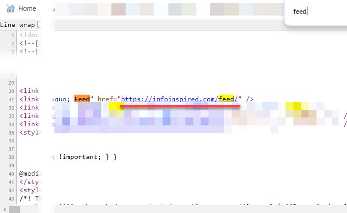
How do I find the URL for use in the IMPORTFEED function?
The easiest way is to open your favorite website in your browser, right-click, and select “View Page Source.” Then search for “feed.”

query: Specifies what data to fetch from the RSS/Atom feed URL. The default query is ‘items’. Here are the supported queries:feed: Returns a single row containing feed information, including the title, description (tagline), and URL.items: [Default] Returns a full table containing items from the feed, such as the post title, author name, URL of the post, date created, and content summary.items title: Returns post titles.items summary: Returns summaries of posts.items url: Returns URLs of posts.items created: Returns creation dates of posts.
headers: FALSE by default. Specifies whether to include column headers as an extra row on top of the returned value.num_items: The IMPORTFEED function fetches all items currently published on the feed. You can control the number of items fetched by specifying this parameter.
Example:
=IMPORTFEED("https://infoinspired.com/feed/", "items", TRUE, 5)The Best Way to Use the IMPORTFEED Function in Google Sheets

Follow the steps below to easily use the IMPORTFEED function in Google Sheets:
Step 1: Adding Field Labels (Row Headers)
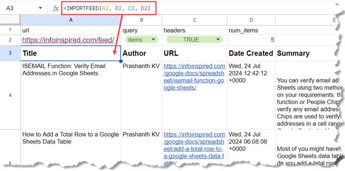
Enter the following IMPORTFEED parameters in cells A1:D1:
url | query | headers | num_items
Step 2: Fetch the RSS/Atom Feed URL
Enter the feed URL, for example, https://infoinspired.com/feed/, in cell A2.
Step 3: Create a Drop-down to Switch Between Query Arguments
- In cell B2, click Insert > Drop-down and create a drop-down list with the following items:
feed,items,items title,items summary,items url,items created. - If you are unfamiliar with this process, follow these steps to create the drop-down:
- Enter the above items in cells B2:B7.
- Select cells B2:B7.
- Click Insert > Drop-down, then click the Done button.
- Select cells B3:B7 and hit the delete key on your keyboard.
- Re-select cells B3:B7, click Insert > Drop-down, then click the Remove Rule button.
Step 4: Create a Drop-down with TRUE or FALSE Values
In cell C2, create a drop-down list with TRUE and FALSE values.
Step 5: Enter the Number of Items
Enter 1 in cell D2 to specify the number of items to display.
Now you are ready to use the IMPORTFEED function. In cell A3, enter the following formula:
=IMPORTFEED(A2, B2, C2, D2)This formula will fetch data based on the values selected or entered in cells A2:D2.
My recommended settings are items in B2 and TRUE in C2. The value in D2, which determines the number of items to fetch, can be set according to your preference.
Looking for a template? Here it is!
How to Aggregate Feeds in Google Sheets
If you want to get recent items from multiple websites, you might typically use a feed aggregator. Here’s how to use the IMPORTFEED function for feed aggregation in Google Sheets.
For a few feeds:
You can use the VSTACK function with the following syntax:
=VSTACK(IMPORTFEED("url_1",,TRUE, 2), IMPORTFEED("url_2",,FALSE, 2))Replace url_1 and url_2 with your RSS/Atom feed URLs. Also, replace the last argument 2 with the number of items you want to retrieve from each website.
For many feeds:
If you have numerous feeds, using VSTACK might not be ideal. In this case, you can use the REDUCE function with IMPORTFEED.
- Enter the feed URLs in cells A1:A.
- Enter the following formula in cell B1:
=REDUCE(TOCOL(,1), TOCOL(A1:A, 1), LAMBDA(acc, url, VSTACK(acc, IMPORTFEED(url,,FALSE, 2))))Limitations of the IMPORTFEED Function
- Throttling: Frequent use of IMPORTFEED may lead to restrictions on data fetching to prevent overloading.
- Data Volume: Handling large feeds can slow down your spreadsheet’s performance.
- Feed Compatibility: Not all RSS or Atom feed formats are supported by IMPORTFEED.
- Manual Refresh: Updates to the feed require manual recalculation or refreshing of the formula.
- Error Handling: IMPORTFEED provides limited error reporting and may not always clearly indicate issues.


How can you have the Date Created and URL columns? I guess this formula depends on the structure of the feed? Some feeds I’ve tried have horrible structure.
Hi, Trang,
Use Query with the IMPORTFEED function.
Example:
=query(IMPORTFEED("https://infoinspired.com/feed/","items",true,10),"Select Col3,Col4")OMG, I don’t even know that this is possible. Totally forgot about Query function. Thanks for sharing.
Hi, how can I feed the data from https://rss.weather.gov.hk/rss/CurrentWeather.xml ?
From its filename, it is XML format, the HTML page is rendered with its XSL. How can I get only the location and degrees?
Best regards,
Kelvin
Hi, Kevin,
Maybe this helps.
=ArrayFormula(transpose(split(ArrayFormula(query(trim(IMPORTFEED("Enter URL Here")),"Select Col5 where Col5 is not null limit 1",0)),";")))Replace ‘Enter URL Here’ with the URL.
Best,
Hi, is there a way to feed a RSS every time a sheet is modified? I need this to create push notifications.
Thanx
Hi, Beppe,
Sorry, I don’t have a solution to offer!
Best,