Learn here the tips on how to increment numbers in grouping in Query in Google Sheets.

You can use the Query function to group and sums data and it’s one of the best function to manipulate data in Google Sheets.

In such grouping, you can insert a column with incrementing numbers similar to the serial number.

When group value in one column changes, the numbering also gets changed. I mean when a new group starts, the numbering starts again from one and then increments.

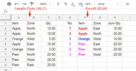
See the below picture. The data is spread across the range A1:C. I have grouped this data based on the value in Column A, then by Column B and summed the value in Column C.

That means, all the same items grouped and if it’s in the same zone, it’s Summed. If you check the output in E1: H you can see a new column with increment numbers, i.e. Column E.

The column E serial number changes when the value (item) in Column F changes. It restarts numbering when value changes in column F.

You can also populate such a column with increment numbers based on grouping if you follow this step by step tutorial. This’s a very detailed tutorial. Here we go!

Increment Numbers in Grouping in Query in Google Sheets

Please go through every step very carefully. If you falter anywhere, refer my Google Sheet that shared at the end of this tutorial.

Step 1: How to Group Data in Google Sheets

We are grouping the above fruits data based on Column A then By B. Column A contains the item name (fruits name) and Column B contains Zone. That means this is an item wise > zone wise summary.

=query(A1:C,"Select A,B,Sum(C) where A<>''group by A,B")

Result:

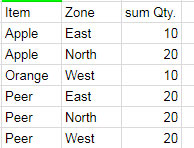
This is our grouped data which is the core in learning how to increment numbers in Grouping in Query in Google Sheets. This data again we will use in our final step at the end of this tutorial.

You can see that the item “Apple” repeats twice because its zone is different. Wherever the item and zone are the same, the formula above groups that rows and sum the Qty.

It’s applicable to all items. Here we want the numbering to start at 1 and it should increment. When the item changes, that means a new group begins, the numbering should restart from 1.

Step 2: Limit the Columns (Keep the Column with Grouped Item Name)

Here the formula is the same as above. But with additional Query, I’ve removed the column 2 and 3.

=query(query(A1:C,"Select A,B,Sum(C) where A<>''group by A,B"),"Select Col1 label Col1''")

Result:

I’ll tell you why this’s required. Please be patient.

Step 3: Unique Grouped Item Names

I am going to apply the Unique function to the above Step 2 result. Here we can use the same formula 2. Here I only want the unique names.

How to return unique names in Query? Just use the Unique function with Query as below.

=unique(query(query(A1:C,"Select A,B,Sum(C) where A<>''group by A,B"),"Select Col1 label Col1''"))

Result:

Step 4: Countif on Queried Data in Google Sheets

Now time to tell you why the above step 2 and 3 is required. I am going to use the above two formulas in Google Sheets Countif function as arguments.

Syntax: COUNTIF(range, criterion)

In the below formula, I’ve used the formula in Step 2 above as the Countif range and Step 3 formula as the Countif criterion.

Check the above Step 3 output. There are 3 criteria. So we should use the ArrayFormula together with Countif. It would be like;

ArrayFormula(COUNTIF(range, criterion))

Here is that formula.

=ArrayFormula(countif(query(query(A1:C,"Select A,B,Sum(C) where A<>''group by A,B"),"Select Col1 label Col1''"),unique(query(query(A1:C,"Select A,B,Sum(C) where A<>''group by A,B"),"Select Col1 label Col1''"))))

Result:

This formula counts how many times each grouped item appears. That means how many times each item in Step 3 result appears in Step 2 result.

Here 2 in the result means, the item Apple repeats two times, 1 means Orange repeats 1 time and the last number 3 indicates the item Peer repeats three times.

This is the logic. If the number of repetition is three I want to increment that number to three times. If it’s one no increment.

Step 5: Increment Numbers for Grouped Data Using Column Function

Before going to this formula, see one example. Imaging that our Step 4 formula result is in the range N10: N12.

=ArrayFormula(if(COLUMN(A1:AE1)<=N10:N12,COLUMN(A1:AE1),""))

If so, this formula would return the result as below. Here the Column function together with ArrayFormula can return column numbers up to the column AE1 such as 1,2,3….31. AE1 is a random column number.

How to determine which column reference to be used or how I come to AE1? See the above Step 4 result. There the maximum number is 3 in the range. So you can use A1: C1 in the above formula to return the number 1,2 and 3.

But our formula is covering infinite ranges. We are unsure about the number of rows in our fruit data. So to get more flexibility I have used a higher column AE1.

It has no impact on the formula as the formula would automatically restrict the column numbering expanding based on the maximum number in N10: N12.

The above formula simply increments the grouped numbers in Step 4 result row-wise. If you refer the screenshot in Step 4, you can understand it.

Here instead of the temporary range N10: N12 we can use the formula in Step 4. The result would be the same.

=ArrayFormula(if(COLUMN(A1:AE1)<=ArrayFormula(countif(query(query(A1:C,"Select A,B,Sum(C) where A<>''group by A,B"),"Select Col1 label Col1''"),unique(query(query(A1:C,"Select A,B,Sum(C) where A<>''group by A,B"),"Select Col1 label Col1''")))),COLUMN(A1:AE1),""))

Step 6: Join Numbers in Different Rows Together

We are inching towards our final steps to create a formula that increment numbers in Grouping in Query in Google Sheets.

Now we have incrementing numbers for each grouped item in individual rows. But we want it in column wise that also in one single column. So we should first join the numbers together and then split and transpose them.

In this step, we are only joining the increment numbers in different rows together. In the next step, we can learn how to split these numbers and transpose them into one single column.

=ArrayFormula(CONCATENATE("-"&ArrayFormula(if(COLUMN(A1:AE1)<=ArrayFormula(countif(query(query(A1:C,"Select A,B,Sum(C) where A<>''group by A,B"),"Select Col1 label Col1''"),unique(query(query(A1:C,"Select A,B,Sum(C) where A<>''group by A,B"),"Select Col1 label Col1''")))),COLUMN(A1:AE1),""))))

Here I’ve just added the CONCATENATE function with the formula in Step 5 and used “-” as the delimiter to join the text.

Result:

Step 7: Split Increment Numbers to Single Column

We have already created the increment numbers in the grouping. But it’s not in the correct form. We need to apply some cleaning to the above result.

={"Serial No.";TRANSPOSE(SPLIT(ArrayFormula(CONCATENATE("-"&ArrayFormula(if(COLUMN(A1:AE1)<=ArrayFormula(countif(query(query(A1:C,"Select A,B,Sum(C) where A<>''group by A,B"),"Select Col1 label Col1''"),unique(query(query(A1:C,"Select A,B,Sum(C) where A<>''group by A,B"),"Select Col1 label Col1''")))),COLUMN(A1:AE1),"")))),"-"))}

Here I only want to use the SPLIT function to split the numbers based on delimiter “-“, then Transpose it into one column. Additionally, I’ve added the text “Serial No.” as the column label.

Result:

This is the increment number that changes based on Grouping in Google Sheets. Yup! you have already learned how to increment numbers in Grouping in Query in Google Sheets. Now you only need to join this column with the grouped data in Step 1.

So we want to join the Formula in Step 1 with Formula in Step 7 to get a side by side result. We can use the Curly Braces to join both the formulas. See Step 8 below for details.

Step 8: Final Formula that Increments Numbers in Grouping in Query in Google Sheets

Here is our final formula.

={{"No.";TRANSPOSE(SPLIT(ArrayFormula(CONCATENATE("-"&ArrayFormula(if(COLUMN(A1:AE1)<=ArrayFormula(countif(query(query(A1:C,"Select A,B,Sum(C) where A<>''group by A,B"),"Select Col1 label Col1''"),unique(query(query(A1:C,"Select A,B,Sum(C) where A<>''group by A,B"),"Select Col1 label Col1''")))),COLUMN(A1:AE1),"")))),"-"))},query(A1:C,"Select A,B,Sum(C) where A<>''group by A,B")}

That’s all. This way you can increment numbers in Google Sheets Query. When grouping changes the numbering again starts from 1.

As promised, here is my sample sheet where I have added and highlighted each and every formula mentioned in this post. So you can understand how individual formulas work before adding them one by one in each step to form a complex formula.

As instructed, once completed this tutorial, follow my shared spreadsheet so that you can easily learn the steps involved to create a formula that increment numbers in Grouping in Query in Google Sheets.