


")


")

")
")
 in Excel & Google Sheets")


When working with spreadsheets, it’s common to highlight duplicates in Google Sheets to catch repeated entries, errors, or data quality issues. Normally, duplicates are identified when the same value appears more than once in a column or row.
But what if you only want to highlight duplicates based on specific conditions? For example:
- When certain products are purchased together.
- When an item is repeated more times than allowed.
- When duplicates should only be flagged under business rules, not just raw repetition.
That’s where conditional duplicate highlighting comes in.
In this guide, you’ll learn step by step how to highlight duplicates in Google Sheets with conditions using custom formulas and conditional formatting. This goes beyond the basic “highlight duplicates” feature and gives you full control over which entries should actually be flagged.
Example of Conditional Duplicate Highlighting in Google Sheets
Let’s say column A contains the name of the person ordering books, and column B lists the books they ordered.
We have limited stock of Book A and Book B, so a person can order either one, but not both.
Sample Data:
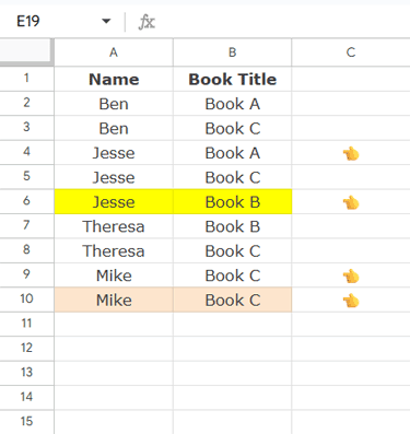
- Jesse ordered both Book A and Book B → This should be flagged.
- Mike ordered Book C twice → This can also be flagged if we want to catch repeated entries.
This is where conditional duplicate highlighting shines.
How to Highlight Duplicates with Conditions in Google Sheets
Follow these steps:
- Select your range →
A2:B - Go to Format > Conditional formatting
- Under Format rules, choose Custom formula is
- Enter this first formula:
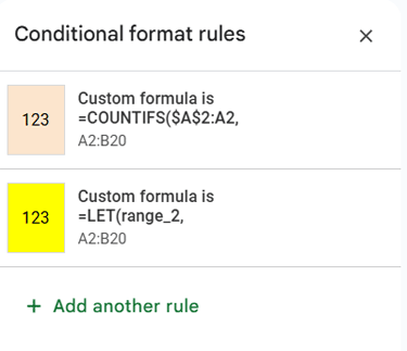
=COUNTIFS($A$2:A2, $A2, $B$2:B2, $B2)>1👉 This rule highlights regular duplicates.
Set the formatting style to “Light Orange”.
- Now, click Add another rule and enter this formula:
=LET(
   range_2, ARRAYFORMULA(REGEXREPLACE($B$2:B2, "Book A|Book B", "x")),
   COUNTIFS($A$2:A2, $A2, range_2, CHOOSEROWS(range_2, -1))>1
)
👉 This is the conditional rule that actually highlights conditional duplicate entries.
Set the formatting style to Yellow.
Why You Need Two Rules for Duplicate Highlighting
The second formula conditionally flags duplicates. On its own, though, it would also highlight regular duplicates. That’s why we add the first formula — it applies a different color, making it easy to tell them apart.
Formula Breakdown for Conditional Duplicate Highlighting
Formula 1: Highlight Regular Duplicates
=COUNTIFS($A$2:A2, $A2, $B$2:B2, $B2)>1This checks if the same person ($A$2:A2) ordered the same book ($B$2:B2) more than once.
Formula 2: Highlight Conditional Duplicates
=LET(
   range_2, ARRAYFORMULA(REGEXREPLACE($B$2:B2, "Book A|Book B", "x")),
   COUNTIFS($A$2:A2, $A2, range_2, CHOOSEROWS(range_2, -1))>1
)
REGEXREPLACE($B$2:B2, "Book A|Book B", "x")→ replaces both Book A and Book B with a placeholder"x".ARRAYFORMULA(...)→ applies this replacement across the entire column range.LET(range_2, ...)→ stores the modified list asrange_2.CHOOSEROWS(range_2, -1)→ selects the current row’s value from that modified list.COUNTIFS($A$2:A2, $A2, range_2, CHOOSEROWS(...))>1→ checks if the same person has already ordered an"x"(meaning Book A or Book B).
👉 Flags conditional duplicates (e.g., Book A + Book B = treated as two "x" orders).
Extending the Formula for More Conditions
You can add more conditions by updating the REGEXREPLACE pattern:
"Book A|Book B|Book W"👉 To make it case-insensitive and exact match only, use:
"(?i)^(Book A|Book B|Book W)$"Final Thoughts
Highlighting conditional duplicates in Google Sheets gives you more flexibility than the standard duplicate highlighting feature. By combining COUNTIFS, REGEXREPLACE, and conditional formatting, you can enforce business rules — like limiting certain products or flagging over-purchases — directly in your sheet.
Once you understand the logic, you can adapt these formulas to match your own conditions, whether that’s products, dates, or any other business rule.