If you’ve tried adding a running total to a Pivot Table in Google Sheets, you’ve probably discovered that it simply doesn’t work—no matter what settings you try.

Running totals are not supported natively in Google Sheets Pivot Tables. Unlike Excel, Google Sheets does not offer a built-in “Show values as running total” option.

But there is a reliable workaround.

By calculating the cumulative total in the source data using a helper column, you can display a correct running total inside a Pivot Table using the MAX aggregation.

This tutorial shows two proven methods:

• Running total grouped by rows
• Running total grouped by rows and columns

Quick Answer: Running Total in Google Sheets Pivot Table

Google Sheets Pivot Tables cannot calculate running totals internally.

Workaround:

1. Sort the source data in the same order as Pivot Table grouping
2. Add a helper column with an ARRAYFORMULA
3. Calculate cumulative totals using SUMIFS
4. Add the helper column to the Pivot Table
5. Summarize it using MAX

This approach works consistently and supports grouping, filtering, and drill-down.

Why Running Totals Don’t Work in Google Sheets Pivot Tables

Pivot Tables summarize aggregated values, not row-by-row calculations. A running total requires awareness of previous rows, which Pivot Tables do not track.

This causes common issues such as:

• Missing months not carrying forward values
• Blank cells breaking cumulative sequences
• Incorrect totals when grouping by multiple fields

To solve this, the cumulative logic must exist before the Pivot Table is created.

Key Rules Before Adding a Running Total

Before implementing a running total, ensure the following:

• Source data is sorted in the same order as Pivot Table grouping
• The running total is calculated in a helper column
• The last grouping field is excluded from the formula
• Use MAX, not SUM, inside the Pivot Table
• Avoid calculated fields — they won’t work for cumulative totals

Example 1: Running Total in Google Sheets Pivot Table (Grouped by Rows)

Sample Data Structure

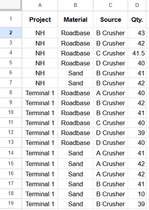
The sample data used in this example contains the following columns:

• Project
• Material
• Source
• Qty

You can copy the sample data by clicking the button below and follow along with this tutorial step by step.

Copy Sample Sheet

Step 1: Create the Pivot Table

1. Select the range A1:E
   (Column E is currently empty and will be used for the helper column.)
2. Go to Insert → Pivot Table
3. Choose Existing sheet, then select cell G1
4. Click Create
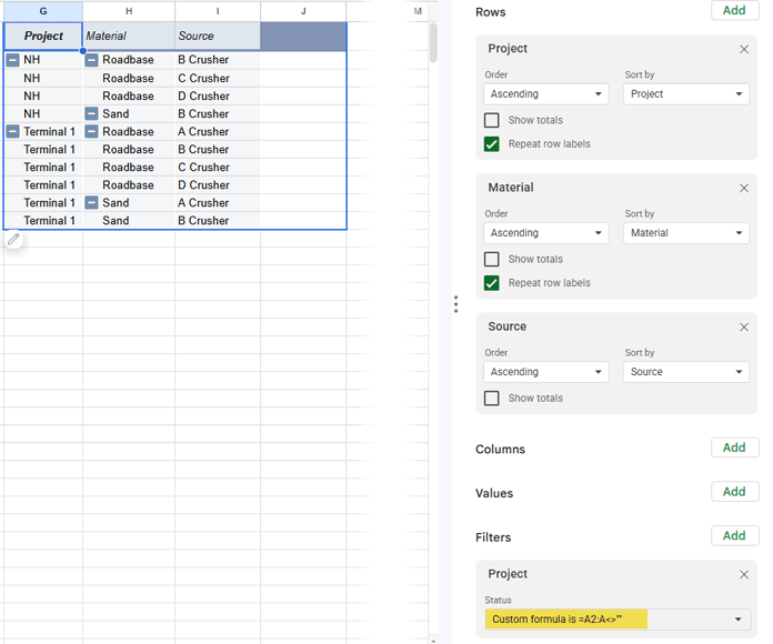
5. In the Pivot Table editor panel, add the following fields:
   • ROWS: Project → Material → Source
   • Disable Show totals for each row field
   • (Optional) Enable Repeat row labels
6. Add Project to the FILTERS section to exclude blank rows.
   After adding it, apply the following Custom formula to remove empty rows:
   =A2:A<>""

If you’re new to Pivot Tables in Google Sheets, refer to Google Sheets Pivot Table Basics & Setup before proceeding.

Step 2: Sort the Source Data

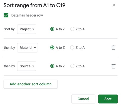
Sort the source data in the same order as the fields in the ROWS section of the Pivot Table.

1. Select the range A1:D
2. Go to Data → Sort range → Advanced sorting options
3. Check Data has header row
4. Sort by:
   • Project — A to Z
   • Material — A to Z
   • Source — A to Z

Important: Sorting the source data is mandatory for accurate running total calculations.

Step 3: Add the Helper Column Formula

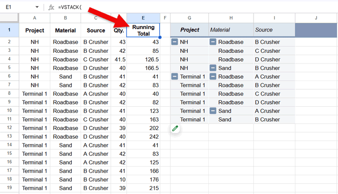
In cell E1, insert:

=VSTACK(
  "Running Total", 
  ARRAYFORMULA(
    MAP(
      A2:A, 
      B2:B, 
      LAMBDA(a, b, IF(a="", ,
        SUMIFS(D2:D, A2:A, a, B2:B, b, ROW(A2:A), "<="&ROW(a)))
      )
    )
  )
)

You don’t need to fully understand the formula to use this method — you only need to adjust the column references.

How the Formula Works

• Groups the data by Project and Material
• Accumulates values row by row to generate a running total
• Excludes Source, which is the last grouping field used in the Pivot Table
  (This is important—running total formulas must omit the last row field to work correctly.)
• Uses row numbers to determine which values are included in the cumulative sum

Adjusting the Formula for More or Fewer Grouping Fields

If you add or remove grouping fields:

• Add or remove the corresponding arrays in the MAP function
• Add or remove the matching criteria inside SUMIFS

Always ensure that:

• The last Pivot Table row field is excluded from the running total calculation

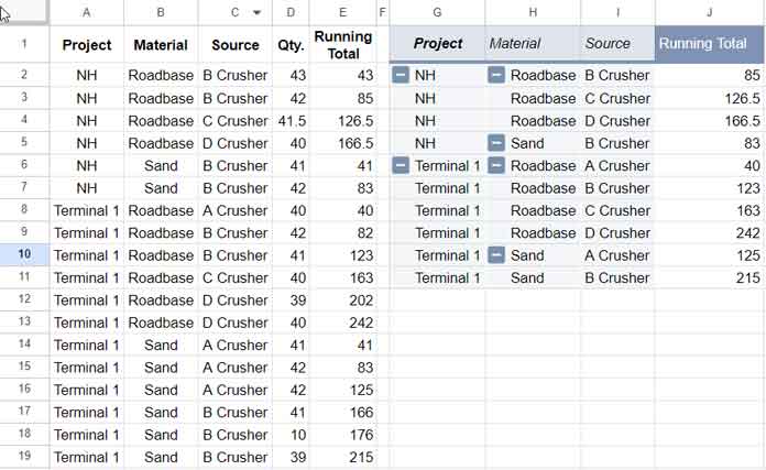
Step 4: Add Running Total to the Pivot Table

1. Open Pivot Table editor (if the sidebar panel is closed, you can click the pencil icon at the lower left of the pivot table by moving your cursor over it)
2. Add Running Total under VALUES
3. Set Summarize by → MAX
4. Rename the header in cell J1 to Running Total

✅ You now have a correct running total inside the Pivot Table.

Example 2: Running Total Grouped by Rows and Columns

When grouping data by columns, running totals appear horizontally (across columns) rather than vertically.

Sample Data Structure

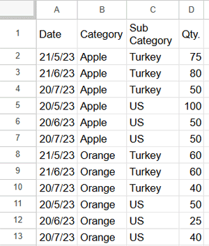
The sample data used in this example contains the following column structure:

• Date
• Category
• Sub-Category
• Qty

You can find this sample data in the same sample sheet used for Example 1 to follow along with this example.

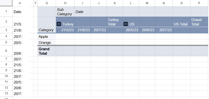
Pivot Table Setup

Configure the Pivot Table fields as follows (ensure columns A to E are selected to accommodate the helper column):

• ROWS: Category
• COLUMNS: Sub-Category → Date
• FILTERS: Category

After adding Category to the FILTERS section, apply the following Custom formula to remove empty rows:

=B2:B<>""

Sort the Source Data

Sort the source data in the following order:

1. Category
2. Sub-Category
3. Date

Helper Column Formula

In cell E1, insert the following formula:

=VSTACK(
  "Running Total", 
  ARRAYFORMULA(
    MAP(
      B2:B, 
      C2:C, 
      LAMBDA(b, c, IF(b="", ,
        SUMIFS(D2:D, B2:B, b, C2:C, c, ROW(A2:A), "<="&ROW(b))))
      )
  )
)

This formula calculates a running total grouped by Category and Sub-Category, while excluding Date, which is the last grouping field in the Pivot Table.

Final Pivot Table Settings

1. Right-click any date inside the Pivot Table
2. Select Create pivot date group → Month
3. In the Pivot Table editor, add Running Total under VALUES
4. Set Summarize by → MAX
5. Rename the column header to Running Total

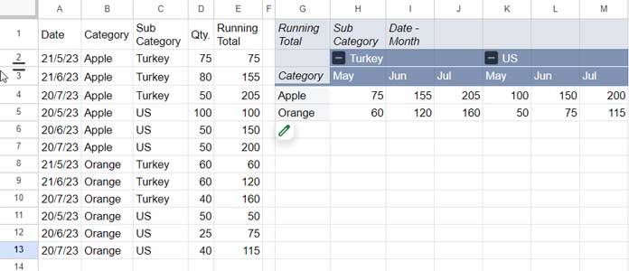
Important Note

When grouping by both ROWS and COLUMNS, use only one field under the ROWS section. Adding additional row fields will create drill-down levels that make horizontal running totals difficult to interpret.

Common Mistakes to Avoid

• ❌ Not sorting source data
• ❌ Using SUM instead of MAX
• ❌ Including the last grouping field in the formula
• ❌ Using calculated fields for cumulative totals
• ❌ Expecting blank periods to auto-carry values
  If a period has no underlying data, it will appear as a blank cell, but the running total does not reset or break. The cumulative value continues correctly in the next available period.

When This Method Is Not Ideal

Avoid this approach if:

• You need Excel-style running totals
• Missing dates must auto-fill values
• You require row-level calculations inside the Pivot Table

In such cases, a QUERY-based report is often a better choice.

Key Takeaways

• Google Sheets Pivot Tables cannot calculate running totals directly
• Helper columns are required
• Sorting source data is non-negotiable
• Exclude the last grouping field in the formula
• Always summarize running totals using MAX

Part of the Hub

This tutorial is part of the Pivot Table Calculations & Advanced Metrics in Google Sheets series, where we cover advanced techniques that go beyond standard Pivot Table features.