There are different methods to calculate and return a horizontal running total in Google Sheets. We can group them into two categories.

They are non-array (1) and array (2) options.

• Non-Array Options.
  • Totaling numbers with plus signs.
  • Using the SUM function by setting the reference to absolute and relative. ✅
• Array Options.
  • SUMIF formula. ✅
  • MMULT formula.
  • DSUM formula.
  • SCAN formula. ✅

You will find all of the above formulas below, and I hope that will help you understand when someone uses them. But the ticked ones are the simplest among them.

What is meant by horizontal running total?

A horizontal running total is the cumulative sum of a value and all previous values in the row.

E.g.:-

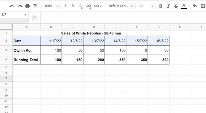
Assume we are selling white pebbles, and we have recorded the sales data of last week in B3:G5 in Google Sheets.

It’s 100 (B3), 50 (C3), 50 (D3), 150 (E3), 0 (F3), and 30 (G3).

We expect the output of 100, 150, 200, 350, 350, and 380 in B4:G4 as per the below screenshot.

Horizontal Running Total – Easiest Array and Non-Array Formulas

Non-Array Formula: ✅

=sum($B$3:B3)

In cell B4, key in the above formula and drag the fill handle across to copy it.

While doing so, the first cell reference in the formula will stay the same because of the absolute cell reference in the first part of the range.

The range reference in the formula changes as follows.

Array Formula: ✅

=ArrayFormula(sumif(column(B3:G3),"<="&column(B3:G3),B3:G3))

Empty the range B4:G4 and enter the above SUMIF in B4.

It will return the horizontal running total of the sales quantity of pebbles in the range B4:G4 from B4.

Now, look at any dates in row # 2 and the corresponding horizontal running total in row # 4.

You can get the total of white pebbles’ sales up to that date.

Explanation of the Array Formula

To explain the formula, I feel it’s better to start with the syntax. Here we go!

Sumif Syntax: SUMIF(range, criterion, [sum_range])

Here are the formula elements representing the arguments in SUMIF.

range – column(B3:G3)

criterion – "<="&column(B3:G3)

sum_range – B3:G3

It means to sum the range B3:G3 if column(B3:G3) <= column(B3:G3).

To understand, let me show you how the formula evaluates the condition in cell C4. You can guess the rest.

It’s like 2<=3, 3<=3, 4<=3, 5<=3, 6<=3, and 7<=3.

The output will be TRUE in the first two cells and FALSE in the next 4 cells.

You can find the other methods to calculate the horizontal running total in Google Sheets below.

You May Also Like:- Normal and Array-Based Running Total Formula in Google Sheets.

Other Horizontal Running Total Formulas for Advanced Users

You can skip the following formulas, except SCAN, as I find them complex compared to the above. Also, I am not going into the explanation part of them.

Still, I am providing it as, at some point in time, you can see some of them, especially the MMULT, in Sheets.

The sample data is the same for the below formulas, i.e., the supply quantity of pebbles in B3:G3.

Non-Array Formula:

=n(A4)+B3

Insert it in cell B4 and copy-paste it across.

Array Formula Alternatives to Horizontal Running Total:

To return the horizontal running total in B4:G4, enter the below MMULT in cell B4.

=ArrayFormula(mmult(B3:G3,IF(column(B3:G3)>=transpose(column(B3:G3))=TRUE,1,0)))

You must delete any values in the output range first to avoid the #REF error.

Here is the DSUM alternative, and follow the above array formula instructions when using it also.

=ArrayFormula(dsum({B3:G3;transpose(if(sequence(6,6)^0+sequence(6,1,column(B3)-1)>=column(B3:G3),B3:G3))},sequence(1,6),{if(,,);if(,,)}))

Finally, here is the latest one using the SCAN Lambda formula. ✅

=scan(0,B3:G3,lambda(a,v,a+v))

That’s all. Thanks for the stay. Enjoy!