


")


")

")
")
 in Excel & Google Sheets")


To conditionally format or highlight up and down in ranking in Google Sheets, follow two steps:
- Rank the data for two different periods
- Consolidate (or compile) the ranked data
Once these steps are done, you can highlight increases and decreases in ranking between the two periods.
Use red to highlight a drop in ranking and green for an improvement. Want to see how it looks? Scroll down to the final screenshot.
Let me first walk you through the two steps in detail.
Rank Data in Google Sheets
You can use either the RANK or RANK.AVG function in Google Sheets. For this example, I’m using the RANK function.
Are you new to these functions and want to know the difference?
Check out my Google Sheets function guide — both functions are covered there along with many others.
Datasets to Consolidate and Highlight Up and Down in Ranking
To test this, you could use:
- Sales volume in two different months
- Average marks of students across two exams
- FIFA world rankings (men’s), comparing current and previous periods
I’ll go with the last example — using FIFA world rankings — to demonstrate how to highlight up and down movements in ranking in Google Sheets.
Note: The sample data below is for demonstration only. You can refer to this Wikipedia article or the official FIFA site for accurate data.
Sheet1: Top 10 FIFA Rankings – April 2025
=ArrayFormula({"Rank"; RANK(C2:C11, C2:C11)})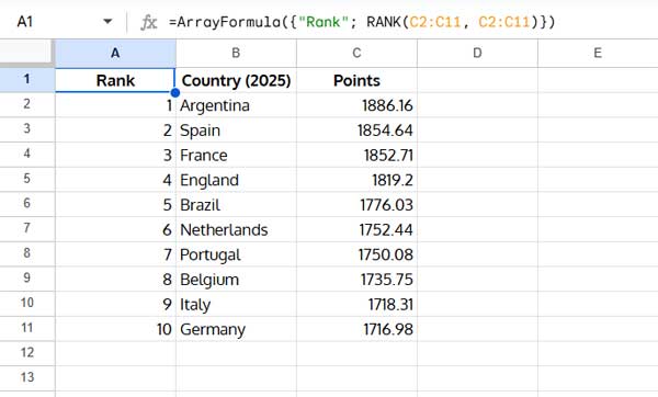
In this sheet, I’ve used the RANK function in cell A1 to calculate the rankings based on points (in column C).
Since the data is sorted by points, the ranking in column A will naturally appear in order — 1, 2, 3, and so on. Sorting by points is necessary here to ensure the rank values align visually with the order of teams based on their performance.
You can rank a specific value (e.g., C2) or an entire range (e.g., C2:C11). The example above ranks all values using ArrayFormula with RANK.
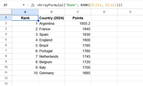
Sheet2: Top 10 FIFA Rankings – End of 2024
Same setup — I’ve used the same RANK formula to rank countries based on their points. As in Sheet1, the data is sorted by points to ensure the ranking appears in the correct top-down order (1, 2, 3, etc.).
Consolidate Data to Compare Rankings in Two Periods
Now, let’s combine the data from both sheets in a third sheet (Sheet3) to make comparisons.
Sheet3: Combine Sheet1 and Sheet2
In cell A1 of Sheet3, enter the following formula:
={Sheet1!A1:B11, Sheet2!B1:B11}| Rank | Country (2025) | Country (2024) |
| 1 | Argentina | Argentina |
| 2 | Spain | France |
| 3 | France | Spain |
| 4 | England | England |
| 5 | Brazil | Brazil |
| 6 | Netherlands | Portugal |
| 7 | Portugal | Netherlands |
| 8 | Belgium | Belgium |
| 9 | Italy | Italy |
| 10 | Germany | Germany |
This formula pulls:
- Columns A and B (Rank + Country) from Sheet1 (current period)
- Column B (Country) from Sheet2 (previous period)
I’ve intentionally skipped the rank column from Sheet2 to avoid duplication.
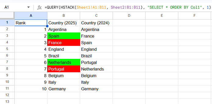
Highlight Up and Down in Ranking (Conditional Formatting)
We’ll now use custom conditional formatting to highlight changes in rank.
Note: If two countries share the same rank in either period (i.e., a tie in points), it may affect how changes in ranking are interpreted. For more accurate comparisons, consider adding a secondary sorting factor (such as alphabetical order or team ID) to break ties consistently.
In columns B and C, you’ll see country names from the current and previous rankings, respectively. We’ll highlight names in column B based on how their ranking changed compared to column C.
Custom Conditional Formatting Rules
- ✅ If a country moved up in column B (compared to C) → highlight green
- ➖ If there’s no change, leave it uncolored
- 🔻 If a country moved down in column B (compared to C) → highlight red
For example, if “Spain” moved up in the rankings, cell B3 should be highlighted in green.
Find and Highlight a Rise in Ranking (With Explanation)
To check whether a country moved up, use this formula:
=VLOOKUP(B2, {C$2:C$11, A$2:A$11}, 2, 0) > A2VLOOKUP(B2, {C$2:C$11, A$2:A$11}, 2, 0)looks up the previous rank of the country in B2- If that previous rank is greater than the current rank in A2, the country has moved up
To test this, enter the formula in cell D2 and copy it down (you can delete it later).
Wherever it returns TRUE, the country improved in rank.
- Select the range
B2:B11 - Go to Format > Conditional formatting
- Use the above formula as a custom formula
- Choose green fill for the “rise” rule
How to Find a Fall in Ranking
To highlight countries that moved down, tweak the formula slightly:
=VLOOKUP(B2, {C$2:C$11, A$2:A$11}, 2, 0) < A2This checks if the previous rank is less than the current — indicating a fall.
Use this as the second conditional formatting rule, and set the fill color to red.
Example: Highlight Up and Down in Ranking in Google Sheets
You’ll now clearly see which countries improved or dropped in the rankings — visually marked with colors.
Bonus Tip: Use This for Non-Rank Data Too
Have you ever tried to highlight changes in row position instead of ranking?
You can apply the same logic:
- Fill column A with sequential numbers using the SEQUENCE function
- Use the same two conditional formatting formulas
- Apply it to a wider range like
B2:B
This allows you to visually track whether a value in column B appears higher or lower compared to column C — a flexible way to highlight up and down movements without actual rank data.
Note: This method works best when both columns contain unique values.
Resources
- Ranking a Non-Existing Number in Google Sheets Data
- How to Rank Group Wise in Google Sheets in Sorted or Unsorted Group
- Highlight Top 10 Ranks in Single or Each Column in Google Sheets
- How to Rank Data by Alphabetical Order in Google Sheets
- How to Rank Text Uniquely in Google Sheets
- How to Use RANK IF in Google Sheets (Conditional Ranking)