We can easily highlight unique top N values in columns or rows in Google Sheets using a combination of the UNIQUE and RANK functions.

Additionally, we can optionally use the COUNTIF function to apply a white fill color to duplicates. Let’s start with an example before moving on to the formulas.

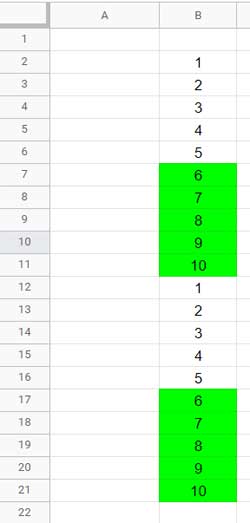
Consider the numbers {1;2;3;4;5;6;7;8;9;10;1;2;3;4;5;6;7;8;9;10} in a column (range B2:B21) in Google Sheets.

If N=5, the unique top N numbers to highlight in B2:B21 will be 10, 9, 8, 7, and 6, not 10, 10, 9, 9, and 8.

Additionally, you may choose whether to apply the fill color to multiple occurrences of the top N numbers. If needed, we can use a COUNTIF rule to exclude duplicates.

Here are examples (screenshots) of single-color highlighting approaches:

• Unique Top 5 (All Occurrences):

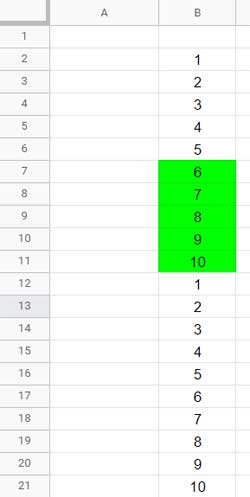
• Unique Top 5 (First Occurrence Only):

Highlight Unique Top N Values in Columns in Google Sheets

Follow these steps to apply conditional formatting:

1. Select Format > Conditional formatting.
2. Under the Single color tab, adjust the settings as follows:
   • Apply to range: B2:B21
   • Format rules: Custom formula is (insert the formula below)
   • Formatting style: Choose a fill color (e.g., Green)
3. Click Done.

All Occurrences:

=RANK(B2, UNIQUE(B$2:B$21))<=5

If you want to apply this rule to an entire column (B2:B), replace B$2:B$21 with B$2:B.

To highlight the unique top 10 numbers instead, replace 5 with 10.

This formula highlights all occurrences of unique top N values.

First Occurrence:

To highlight only the first occurrence, add another condition:

=AND(RANK(B2, UNIQUE(B$2:B$21))<=5, COUNTIF(B$2:B2, B2)<2)

Highlight Unique Top N Values in Multiple Columns

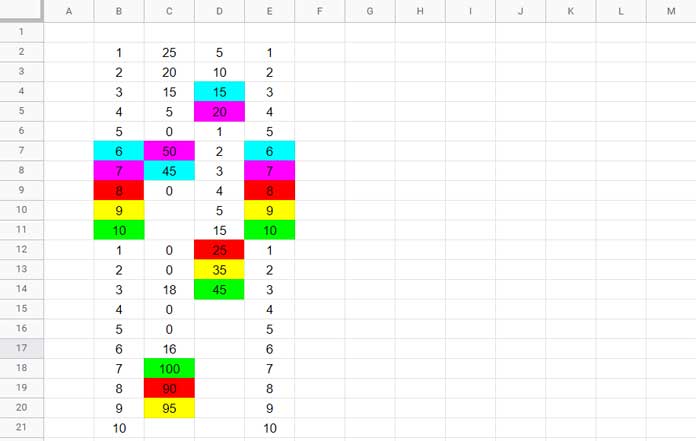
To highlight the largest unique N numbers in each column in B2:E21, update the “Apply to range” field to B2:E21.

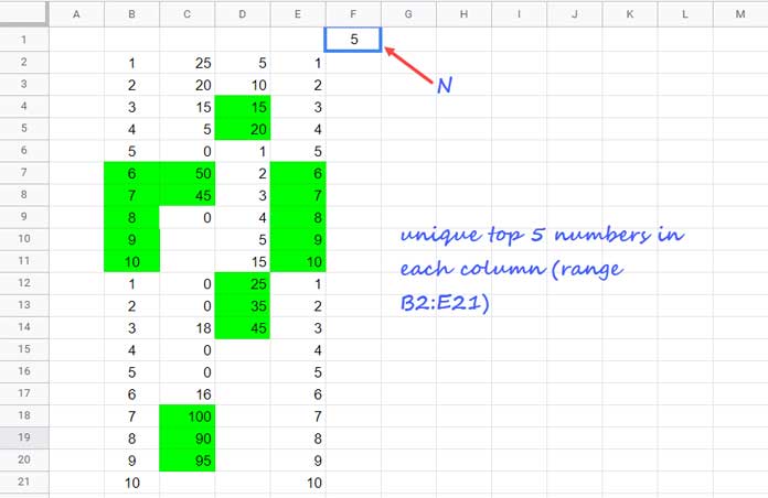
Formula Explanation

• RANK(B2, UNIQUE(B$2:B$21)) ranks the value in B2 among the unique values in B2:B21.
• If the rank is <=5, the formula returns TRUE, highlighting the top 5 unique values.
• To eliminate second and later occurrences, COUNTIF(B$2:B2, B2)<2 ensures that only the first occurrence is highlighted.

Highlight Unique Top N Values in Rows in Google Sheets

We have seen how to highlight unique top N values in columns. What about rows?

For row-based highlighting, use Apply to Range as B2:U2 (or B2:U).

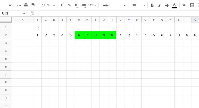
Formula for Unique Top N Values in Rows:

• All occurrences:=RANK(B2, UNIQUE($B2:$U2, TRUE))<=5
• First occurrence only:=AND(RANK(B2, UNIQUE($B2:$U2, TRUE))<=5, COUNTIF($B2:B2, B2)<2)

Additional Tips: Highlight Unique Top N Values with Multiple Colors

If you want to differentiate between unique top N values using different colors, follow these steps:

For Top 1, Top 2, Top 3, etc., create separate rules with different colors:

• Rule 1 (Top 1 Value):=AND(RANK(B2, UNIQUE(B$2:B$21))=1, COUNTIF(B$2:B2, B2)<2)
• Rule 2 (Top 2 Value):=AND(RANK(B2, UNIQUE(B$2:B$21))=2, COUNTIF(B$2:B2, B2)<2)

Continue adding more rules, changing =1 to =2, =3, etc., and selecting different fill colors.

Related Articles

• Highlight Max Value Leaving Duplicates Row-wise in Google Sheets
• How to Highlight the Largest 3 Values in Each Row in Google Sheets
• Highlight Top 10 Ranks in Single or Each Column in Google Sheets