")


")


")

")
")
 in Excel & Google Sheets")


Looking to highlight the lowest value within each group in Google Sheets? This tutorial shows you exactly how to do that using two simple conditional formatting rules.
Let’s say you have a dataset with player names in column A, their ages in column B, and countries in column C. You want to highlight the minimum age for each country—that’s what we’ll demonstrate.
But for simplicity, we’ll use a different example involving fruits and their quantities.
Example: Highlight the Min Value in Each Group in Google Sheets
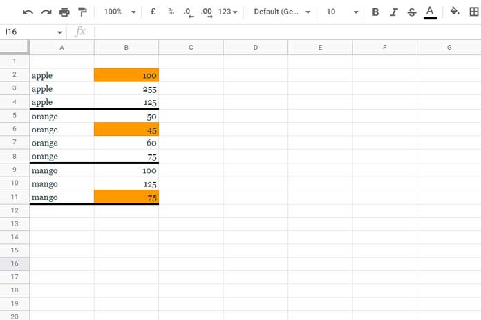
Goal: Highlight the minimum quantity for each fruit in column B, grouped by the fruit name in column A.
Sample Data Range: A2:B20
How to Highlight the Min Value in Each Group in Google Sheets
To highlight the lowest value per group, apply two conditional formatting rules:
Rule #1: Highlight Blank Cells in Column B (Optional)
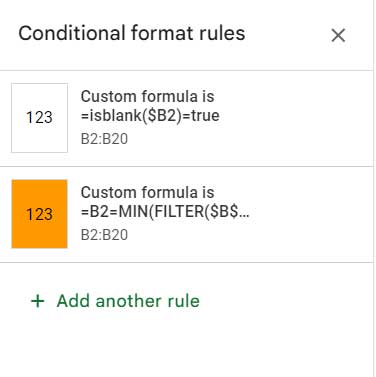
=ISBLANK($B2)Use this rule to apply a white fill color to blank cells, so they don’t get highlighted as if they were the minimum value.
Rule #2: Highlight the Minimum Value in Each Group
=B2=MIN(FILTER($B$2:$B$20, $A$2:$A$20=A2))This formula checks if the value in column B is the minimum among all values in the same group based on the fruit name in column A.
Steps to Apply Conditional Formatting
- Select the range B2:B20.
- Go to Format > Conditional formatting.
- Under “Format cells if,” select “Custom formula is” and paste Rule #1. Choose a white fill color.
- Click “Add another rule”, select “Custom formula is”, and paste Rule #2. Choose an orange fill color.
- Click Done.
Note: Make sure Rule #1 (blank cells) is listed above Rule #2 in the Conditional Format panel to prevent conflicts.
How the Formula Works
In each row, the formula:
=FILTER($B$2:$B$20, $A$2:$A$20=A2)filters the values in column B where the fruit in column A matches the current row. For example, for row 2 (“Apple”), it returns 100, 255, 125.
Then:
=MIN(...)returns the smallest value in that group—in this case, 100.
Finally:
=B2=MIN(...)compares the value in column B to the group’s minimum. If it matches, it returns TRUE, and the cell is highlighted in orange.
Why Rule #1 Is Important
Without Rule #1, blank cells might get highlighted because MIN can return 0 or misinterpret empty values. Rule #1 ensures that blank cells remain unformatted by applying a white background.
Extra Tip: Highlight the Minimum Value in Each Group While Excluding Zeros
If you want to highlight the minimum value in each group but exclude zeros, you can skip Rule #1 entirely and use just this modified formula:
=B2=MIN(FILTER($B$2:$B$20, $A$2:$A$20=A2, $B$2:$B$20>0))How it Works:
- The
FILTERfunction extracts non-zero values in the current group. MINreturns the smallest number greater than 0.- If all values are zero or blank, the formula returns
#N/A, which prevents incorrect highlighting.