")
")


")


")

")
")
 in Excel & Google Sheets")


Want to highlight max values like scores, amounts, or dates in a row or across multiple rows in Google Sheets? Since there’s no built-in rule for this, you can use a custom formula to achieve it. This formula works seamlessly with numbers, dates, and times and adjusts row-wise. Let’s dive into two examples to see how it works.
Example 1: Highlight Max Value in a Row
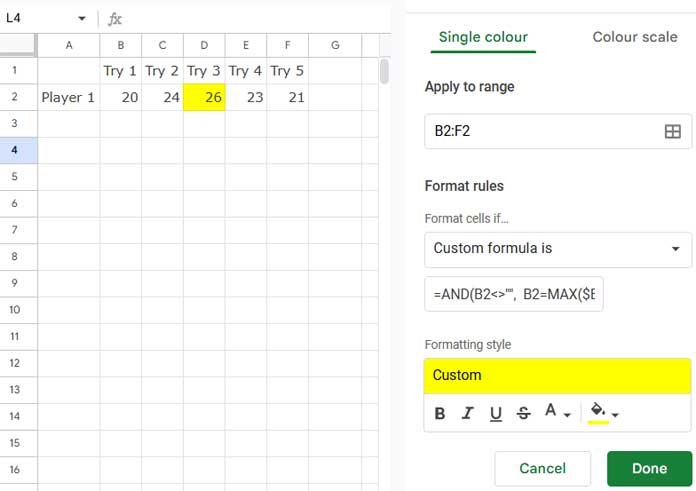
Assume you have the scores of one player in five attempts in the range B2:F2, and you want to highlight the max score. Here is how to do it:
- Select the range B2:F2.
- Click Format > Conditional Formatting.
- Select Custom Formula under Format Rules.
- Enter the following formula:
=AND(B2<>"", B2=MAX($B2:$F2)) - Select the fill color or font color you want to apply to the max value.
- Click Done.
This will highlight the max value in the row.
Formula Breakdown
The formula follows the syntax:
AND(logical_expression1, [logical_expression2, ...])- logical_expression1:
B2<>""– Ensures the cell is not empty. - logical_expression2:
B2=MAX($B2:$F2)– Checks if the value in the cell equals the max value in the range.
If the row is empty, no highlighting will be applied.
Example 2: Highlight the Highest Value in Each Row
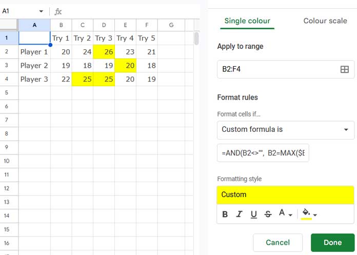
If you want to highlight the max value in each row, simply extend the “Apply to range” selection. No changes to the formula are needed.
For example, assume three players participated in a game and attempted five times each. The scores are in the range B2:F4. Here’s what to do:
- Select the range B2:F4.
- Click Format > Conditional Formatting.
- Use the same formula:
=AND(B2<>"", B2=MAX($B2:$F2)) - Select your desired highlight color.
- Click Done.
The formula will automatically adjust for each row because the MAX function calculates the max value in each row, as the column reference is absolute and the row reference is relative.
Additional Resources
- Google Sheets – Highlight the Max Value in Each Group
- Highlight Max Value Leaving Duplicates in Row Wise in Google Sheets
- Highlight Min Excluding Zero and Blank Cell in Google Sheets
- Skip Duplicates in Min | Small Value Highlighting Row Wise in Google Sheets
- How to Highlight the Min Value in Each Group in Google Sheets