Conditional formatting in Google Sheets can do more than just color-code cells — it can help you spot trends, problems, or unusual patterns without scanning rows manually.

One interesting use case is highlighting duplicates based on date difference.

Normally, duplicate highlighting works by marking any second (or later) occurrence of a value. But what if you only care about duplicates that happen close together in time? That’s where the date difference rule comes in.

Why This Is Useful

Think about running an online bookstore. You might want to see which books are selling repeatedly within a short span — say, within 30 days.

• If Book 1 was sold on Jan 1st and again on Jan 25th, that’s within 30 days → highlight it.
• If the next purchase happens three months later, that one doesn’t need to be highlighted.

This way, your sheet isn’t just showing you duplicates — it’s showing you duplicates that actually matter.

Sample Data

All you need is two columns:

• Date (when something happened)
• Item/Title (what the transaction was for)

Example:

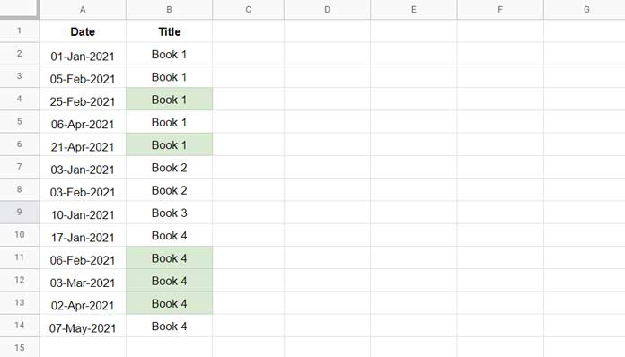
Note: Sorting is not required for the formula to work. However, sorting by Title first and then by Date makes it easier to visually interpret the highlighted duplicates, since you’ll see each highlighted entry right next to its earlier occurrence.

Highlight Duplicates by Date Difference (Conditional Formatting)

Here’s the formula that highlights duplicates within 30 days:

=LET(
   dt, FILTER($A$2:$A, $B$2:$B=$B2, $A$2:$A<$A2), 
   test, $A2-XLOOKUP($A2, dt, dt, ,-1), 
   test<=30
)

What it does

Let’s break the formula down step by step:

1. FILTER($A$2:$A, $B$2:$B=$B2, $A$2:$A<$A2)
   • This looks at the Date column ($A$2:$A).
   • It keeps only the rows where the Item column ($B$2:$B) matches the current row’s item ($B2).
   • It also requires the date to be earlier than the current row’s date ($A$2:$A<$A2).
   • Result: a list of all earlier dates for the same item.
2. XLOOKUP($A2, dt, dt, ,-1)
   • From that list of earlier dates (dt), it pulls the most recent one before the current date.
   • The -1 tells XLOOKUP to return the closest smaller date (the most recent earlier date), not the oldest one.
3. $A2 - (that date)
   • Subtracts the most recent earlier date from the current row’s date.
   • The result is the number of days between this purchase and the last one.
4. test <= 30
   • Finally, it checks if the gap in days is 30 or less.
   • If yes → the cell is highlighted.
   • If no → nothing happens.

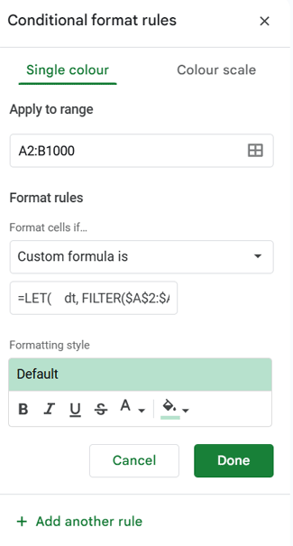
How to Apply It

1. Select your data (e.g., A2:B).
2. Go to Format > Conditional formatting.
3. Under Format rules, choose Custom formula is and paste the formula.
4. Adjust the column references in the formula if your sheet uses different columns.
5. Replace 30 in the formula with the number of days you want to use.
6. Pick a highlight color and hit Done.

Now your duplicates light up only when they’re within the time frame you care about.

Real-World Uses

This trick isn’t just for bookstores. You can use it to:

• Spot repeat customer purchases in a short time frame.
• Track recurring payments.
• See which products are leaving inventory too fast.
• Flag clients who are booking services repeatedly.

Basically, any situation where “duplicates within N days” tells you something meaningful.

Wrap-Up

Highlighting duplicates based on date difference in Google Sheets is a smarter way to work with your data. Instead of marking every duplicate, you only highlight the ones that happen close together — giving you insights into demand, frequency, and patterns you’d otherwise miss.

Related Reading

• Highlight Duplicates in Google Sheets
• Highlight Partial Matching Duplicates in Google Sheets
• Highlighting Visible Duplicates in Google Sheets
• Highlight Max Value Leaving Duplicates Row-Wise in Google Sheets
• How to Highlight Conditional Duplicates in Google Sheets
• How to Find and Highlight Adjacent Duplicates in Google Sheets