Google Sheets allows you to highlight an entire column based on specific conditions using a custom conditional formatting rule.

Depending on your needs, you can define different conditions to highlight columns dynamically. This tutorial will guide you through various examples to help you apply conditional formatting effectively.

Let’s use the timescale (header row of the bar/chart area) in a Gantt chart to demonstrate different highlighting rules. We’ll test with various time units such as days (today), months, and years.

Examples of How to Highlight an Entire Column in Google Sheets

1. Highlight an Entire Column Matching Today’s Date

Assume you have a timescale in B2:O2, where each cell represents a date, and the corresponding bar (plot) area is B3:O17.

To highlight the column that matches today’s date, use this custom formula:

=B$2=TODAY()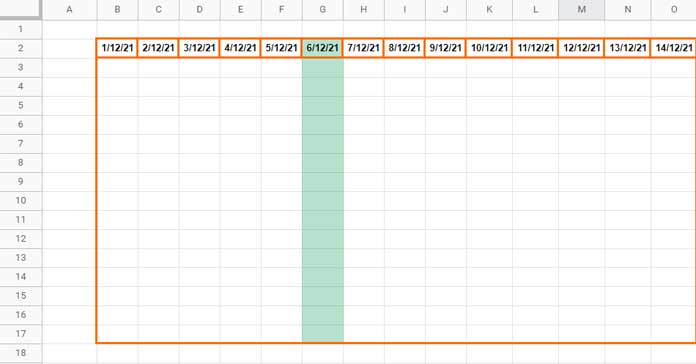

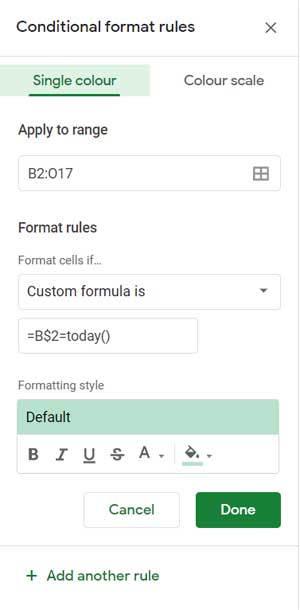
Steps to Apply the Formula:

1. Select B2:O17.
2. Click Format > Conditional formatting.
3. Under Format rules, select Custom formula is.
4. Enter the formula:
   =B$2=TODAY()
5. Choose a fill color (e.g., light gray or yellow).
6. Click Done.

Now, the column corresponding to today’s date will be highlighted.

2. Highlight an Entire Column Matching the Current Month

If your timescale uses date values (e.g., 1/1/2021, 1/2/2021), you can format them to display as month names (e.g., “Jan”, “Feb”) using Format > Number > Custom number format, then enter "mmm" as the format.

If your header row contains such formatted month names, use the following formula to highlight an entire column matching the current month:

=EOMONTH(B$2,0)=EOMONTH(TODAY(),0)

How It Works:

• This formula converts all dates in B2:O2 to the last day of the month.
• It checks if the column header matches the end of the current month instead of today’s exact date.

3. Highlight an Entire Column Matching a Specific Number or Text

You can also highlight columns based on numeric values (e.g., years) or text values (e.g., product names).

• For a specific year: =B$2=2021
• For a specific text value: =B$2="Apple"

4. Highlight an Entire Column for Weekends

To highlight entire columns where the header row contains a weekend date (Saturday or Sunday), use this formula:

=AND(NOT(ISBLANK(B$2)), OR(WEEKDAY(B$2)=7, WEEKDAY(B$2)=1))

• This checks if the header row contains a valid date (not blank).
• It highlights the column if the weekday number corresponds to Saturday (7) or Sunday (1).

If your weekend falls on different days (e.g., Friday-Saturday in some regions), adjust the WEEKDAY numbers accordingly.

For more details on customizing the WEEKDAY function, check my Google Sheets Date Function Guide.

Additional Tips

1. Highlight Columns Within a Specific Date Range

To highlight columns where the date in the header row falls between 3rd December 2021 and 13th December 2021, use this formula:

=AND(B$2>=DATE(2021,12,3), B$2<=DATE(2021,12,13))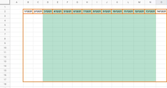

This will highlight multiple columns within the specified date range.

2. Highlight an Entire Column If Any Cell in That Column Matches a Value

If you want to highlight an entire column when a specific value (e.g., “Apple”) appears anywhere in the column (not just in the header row), use this formula:

=MATCH("Apple", B$2:B$17, 0)

• This formula searches for “Apple” in B2:B17 and highlights the entire column if found.
• Adjust the value (“Apple”) or range as needed.

Final Thoughts

Using conditional formatting, you can dynamically highlight an entire column in Google Sheets based on dates, numbers, text, or specific conditions. Try these examples and adapt them to your dataset to improve visibility and data analysis.

Related Resources

• How to Highlight Entire Error Rows in Google Sheets
• Google Sheets: Highlight an Entire Column If Any Cell Has an Error
• Highlight an Entire Row in Conditional Formatting in Google Sheets