You can group data by month and year in Google Sheets in two ways:

1. Using a Pivot Table
2. Using the QUERY function

This tutorial covers both methods, with more emphasis on the QUERY function, as it offers greater flexibility for dashboards and advanced reports.

Why include both month and year?

Why Month-and-Year Grouping Matters

Grouping data by month and year allows you to display results like Jan-2018, which is far more informative than showing just January or month number 1.

In reports such as sales, expenses, fuel consumption, or usage logs, the same month can occur across multiple years. If you group by month alone, values from different years may be incorrectly added together.

• ❌ January 2018 + January 2019 → combined
• ✅ Jan-2018 and Jan-2019 → separate totals

If all records belong to a single year, grouping by month alone is fine. Otherwise, month-and-year grouping is essential.

That said, some users may intentionally want all January values combined across multiple years. In such cases, this type of grouping can be avoided. You can check out my tutorial Creating a Month-Wise Summary in Google Sheets (QUERY Formula) for that approach.

For Pivot Tables, month-only grouping works in a similar way—you simply need to choose the Month option instead of Year-month in the date grouping, which I’ll point out later in this tutorial.

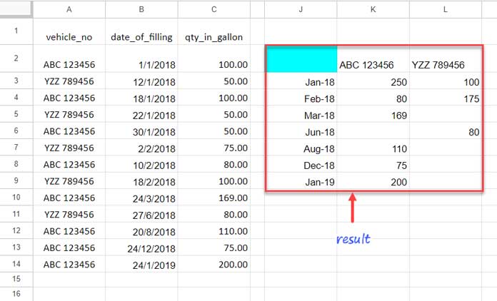
Example Dataset Used in This Tutorial

For this explanation, we’ll use a diesel consumption report.

• Column A: Vehicle number (not unique)
• Column B: Date of fuel filling
• Column C: Quantity in gallons

You can copy the sample sheet provided below and follow along with the steps in this tutorial.

Copy Sample Sheet

This dataset allows us to create a month- and year-wise summary report.

Once you understand this technique, you can apply it to:

• Sales reports
• Purchase orders
• Expense logs
• Material reconciliations

This tutorial is part of our complete Google Sheets Pivot Table Tutorial, covering basics, setup, and advanced date grouping techniques.

Method 1: Group Data by Month and Year Using a Pivot Table

Steps

1. Select the data range A1:C14
2. Go to Insert → Pivot table
3. Choose Existing sheet, enter E1, and click Create
4. In the Pivot Table editor:
   • Add date_of_filling to Rows
   • Add vehicle_no to Columns
   • Add qty_in_gallon to Values
5. Right-click any date value in the Pivot Table
6. Select Create pivot date group → Year-month
   (If you want to group by month only across all years, select Month instead.)

That’s it! Your Pivot Table will now summarize the data by month and year.

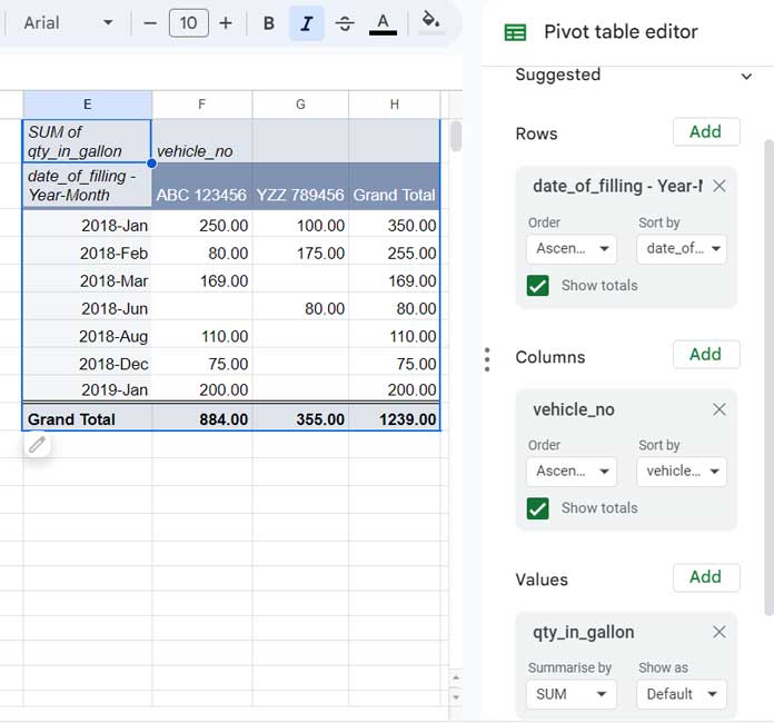
Tip: Always select the actual data range (A1:C14). If you select entire columns (A1:C), you may need to add filters to exclude blank rows.

Method 2: Group Data by Month and Year Using the QUERY Function

Below is the master formula to group data by month and year using QUERY.

Master Formula

=QUERY(
  HSTACK(A2:A14, ARRAYFORMULA(EOMONTH(B2:B14, -1)+1), C2:C14),
  "SELECT Col2, SUM(Col3)
   GROUP BY Col2
   PIVOT Col1
   FORMAT Col2 'MMM-YY'"
)

Notes

• QUERY column identifiers are case-sensitive (Col, not COL)
• If your range is A2:C instead of A2:C14, use:

=QUERY(
  HSTACK(A2:A, ARRAYFORMULA(IFERROR(EOMONTH(DATEVALUE(B2:B),-1)+1)), C2:C),
  "SELECT Col2, SUM(Col3)
   WHERE Col1 IS NOT NULL
   GROUP BY Col2
   PIVOT Col1
   FORMAT Col2 'MMM-YY'"
)

Why the QUERY Formula Works (Important Concept)

Although QUERY is the main function, the core logic comes from the EOMONTH function.

What EOMONTH Does

The formula:

EOMONTH(B2, -1)+1

Converts any date in a month to its beginning-of-month date.

Examples:

• 15/01/2018 → 01/01/2018
• 20/01/2018 → 01/01/2018

This ensures that all dates in the same month and year share a common value, making accurate grouping possible.

Advantages of Converting Dates to the Beginning of the Month

• Eliminates scattered daily dates within a month
• Enables accurate month-and-year grouping
• Maintains correct chronological order
• Allows flexible formatting (MMM-YY, MMM-YYYY, etc.)

Once this concept is clear, the rest of the QUERY formula becomes easy to understand.

When QUERY Is Better Than a Pivot Table

Pivot Tables are easier to create and support totals and subtotals. However, QUERY has distinct advantages:

• Ideal for dashboard reports
• Easier filtering using the WHERE clause
• Grouped dates remain true date values, not text
• Full control over formatting
• Ability to limit results (Top-N reports)

Conclusion

Use a Pivot Table when you need a quick summary with totals and subtotals and minimal setup.

Choose the QUERY function when you’re building dashboards, need advanced filtering, custom formatting, or want full control over how month-and-year grouping behaves.

Both methods support accurate month-and-year grouping—the right choice depends on whether you prioritize ease of use or flexibility and automation.