Is there any particular use of generating 1-12-123-1234 patterns using an array formula in Google sheets?

I think, before giving you the solution, I should answer this question first.

If you know how to generate the said pattern using an array formula, you can transform values in a single column into a database and use them in database functions.

I have recently followed the syntax, transpose(1-12-123-1234_pattern)as a database in DMAX to return Running Max in Google Sheets.

It is simple to get 1-12-123-1234 patterns using a drag-down formula in Google sheets.

But that may not be useful when you require to use the generated values as an expression in an array formula.

Assume you have values in a few rows in column B. It can be text, date, or numbers.

To understand the pattern, I am just using the sequence from 1 to 10 in cell range B2:B11.

In cell D2, insert this TRANSPOSE-based formula and drag it down.

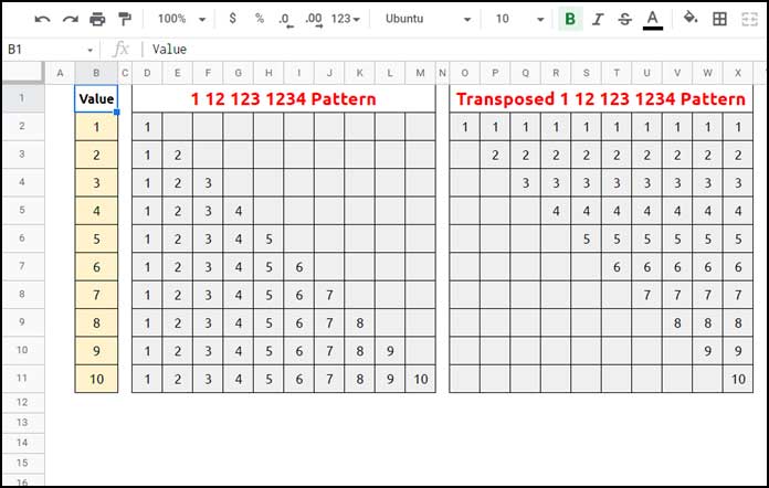
=transpose({$B$2:B2})

It will return or transform the values into the 1-12-123-1234 patterns in cell range D2:M11.

Array Formula to Generate 1-12-123-1234 Patterns in Google sheets

We can use the below IF and SEQUENCE array formula in cell D2 to get the 1-12-123-1234 patterns in cell range D2:M11 in Google Sheets.

=ArrayFormula(
     if(
        sequence(10,10)/sequence(10,10)+sequence(1,10,row(A2)-1)<=row(A2:A11),
        transpose(B2:B11),
     )
)

Note 1:- We can replace sequence(10,10)/sequence(10,10) with sequence(10,10)^0.

It’s a logical test as per the following syntax:

IF(logical_expression, value_if_true,,)

Formula Explanation

We can split the above 1-12-123-1234 Patterns formula into three parts.

There are two logical_expression parts and one value_if_true part.

Here are them.

Part 1 (logical_expression)

We have values in 10 rows in B2:B11. So, I’ve used SEQUENCE to generate sequence numbers in 10 rows and columns.

The below is a sequence matrix fill formula.

sequence(10,10)

Note 2:- When you test, enter it as an array formula (Ctrl+Shift+Enter). So it will become =ArrayFormula(sequence(10,10)). It’s also applicable to the other formula parts below.

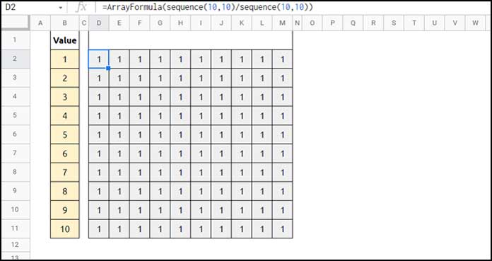
In the next step, I’ve divided the numbers with the same numbers to make all of them 1.

sequence(10,10)/sequence(10,10)

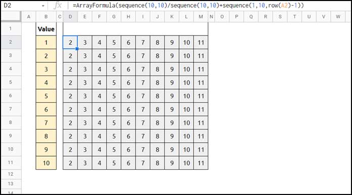
Now we should add sequence numbers 1 to 10 with the above values in each row.

sequence(10,10)/sequence(10,10)+sequence(1,10,row(A2)-1)

To add the numbers 1 to 10, we can use sequence(1,10) but what I have used is sequence(1,10,row(A2)-1).

Because I want to add sequence numbers starting from the first row of the range – 1.

The values are in B2:B11. So I want the numbering to start from 1 to 10.

If it’s from B3:B11, I want the numbering from 2 to 11. That’s why I have used row(A2)-1.

The above logical_expression part plays a vital role in getting the 1-12-123-1234 patterns in Google Sheets.

Part 2 (logical_expression)

We will test whether the values in the above output are less than or equal to the corresponding row numbers in each row. That’s part 2.

sequence(10,10)/sequence(10,10)+sequence(1,10,row(A2)-1)<=row(A2:A11)

In this, the bold formula is part 2.

Note 3:- We can also use the following formula as the logcial_expression (part 1 and 2 combined).

if(row(B2:B11),sequence(1,10,row(A2)))

Part 3 (value_if_true)

If the above (logical_expression) evaluates TRUE, the formula will return transpose(B2:B11), i.e., value_if_true.

This way, we can use an array formula to generate 1-12-123-1234 patterns in Google Sheets.

Transposed 1-12-123-1234 Patterns

We can get the transposed 1-12-123-1234 patterns in the following way (please refer to the range O2:X11 on screenshot # 1).

Just wrap the above formula with TRANSPOSE.

=ArrayFormula(TRANSPOSE(if(sequence(10,10)/sequence(10,10)+sequence(1,10,row(A2)-1)<=row(A2:A11),transpose(B2:B11),)))

It is the type of data that we may sometimes require to solve complex problems using database functions.

At the beginning of this Google Sheets tutorial, I’ve provided the link to one such tutorial.

You may please check that tutorial to understand the usage.

That’s all. Thanks for the stay. Enjoy!