Automatic Gantt Charts with GANTT_CHART in Google Sheets

Managing projects in Google Sheets often requires a clear visual timeline, and Gantt charts are one of the best ways to achieve this. Instead of building them manually with formulas or formatting tricks, you can use the GANTT_CHART named function in Google Sheets to generate them automatically.

This function expands task dates into bars, making it easier to track schedules, compare planned vs. actual progress, and keep projects organized—all with a single formula.

Table of Contents

Data Requirements for the GANTT_CHART Function

Before using the function, make sure your sheet includes:

A task name column and corresponding start date and end date columns
Project start and end dates (timeline)
Project duration in number of days
A status column (optional) for applying different colors to bars based on task status
A timescale that spans from the project start date to the project end date

Once you set these up, you can create an automatic Gantt chart in Google Sheets with the GANTT_CHART named function.

Syntax of the GANTT_CHART Named Function in Google Sheets

GANTT_CHART(start_date_range, end_date_range, from, to, duration, status)

Arguments

start_date_range → The range containing task start dates
end_date_range → The range containing task end dates
from → Timescale start date (cell reference or hard-coded date)
to → Timescale end date (cell reference or hard-coded date)
duration → Total project duration in days
status → Task status column range – if there is no status column, simply refer to the task column

How to Get the GANTT_CHART Named Function

The GANTT_CHART function is a custom named function, not a built-in feature of Google Sheets. You can import it from a ready-made sheet instead of creating it manually.

Make a copy of my sample Google Sheet.
Once copied, the GANTT_CHART named function will automatically be available in that sheet.
You can then use =GANTT_CHART(...) just like a regular formula.

To use the function in another file: open the spreadsheet where you want the function to be available (the destination file). Then go to Data > Named functions > Import functions. In the import dialog, select the copied sample file, choose GANTT_CHART from the list of functions, and click Import. The GANTT_CHART named function will be added to the current (destination) sheet and can be used there immediately.

Steps to Automatically Create a Gantt Chart in Google Sheets

Step 1: Enter task details

In columns A–C, enter your task name, start date, end date, and (optionally) task status.

Example:

Task names, start dates, end dates, and status column entered in Google Sheets for GANTT_CHART function

Step 2: Project timeline

Enter the project start and end dates. For example:

B1 → =MIN(B4:C11)
C1 → =MAX(B4:C11)

This will return the earliest start and latest end dates automatically.

Step 3: Project duration

The duration is the total number of days (inclusive). Enter this in C2:

=C1-B1+1

In our example, the project runs for 79 days.

Project start date, end date, and calculated duration set up in Google Sheets for GANTT_CHART function

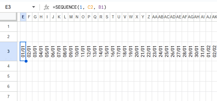
Step 4: Create the timescale

We now need a row of dates across the chart. In E3, enter:

=SEQUENCE(1, C2, B1)

This will expand the project timeline across columns, from the start to the end date. You can optionally format the dates to DD/MM under Format > Number > Custom number format and apply Rotate Up under Format > Rotation for a cleaner Gantt chart view. Further, adjust the column width uniformly to the minimum for a compact timeline display.

Timescale created with SEQUENCE formula showing project dates across columns in Google Sheets

Step 5: Prepare the chart area

For each task row, merge the corresponding timescale columns (E through CE).

Select the range (e.g., E4:CE4)
Click Format > Merge cells > Merge horizontally
Repeat this for each task row. To save time, you can simply copy and paste the first merged row down.

Step 6: Apply the GANTT_CHART function

In E4, enter:

=GANTT_CHART(B4:B11, C4:C11, B1, C1, C2, D4:D11)

Where:

B4:B11 → Task start dates
C4:C11 → Task end dates
B1, C1 → Project start and end dates
C2 → Project duration
D4:D11 → Task status column

Automatic Gantt chart generated with GANTT_CHART named function in Google Sheets

Default Color Schemes for GANTT_CHART in Google Sheets

By default, the GANTT_CHART function supports the following status-based colors:

Complete → #4CAF50 (green)
Upcoming → #90CAF9 (light blue)
In Progress → #FF9800 (orange)
Hold → #9E9E9E (neutral gray)

If you want to show both the planned schedule and the actual progress for each task, the function also supports:

Sch → #9E9E9E (neutral gray)
Actual → #1976D2 (blue)

If no status is provided (either by referring to an empty range or by pointing to the task range itself), all bars appear in dark teal #005B70.

The default background is white, but you can customize these colors by editing the named function under:
Data > Named functions

Look for this part in the formula within Data > Named functions:

{"charttype","bar";
 "color1","white";
 "color2",switch(s,
   "Complete","#4CAF50",
   "Upcoming","#90CAF9",
   "In Progress","#FF9800",
   "Hold","#9E9E9E",
   "Sch","#9E9E9E",
   "Actual","#1976D2",
   "#005B70")}