Google Sheets: Use FVSCHEDULE to Apply Multiple Interest Rates

The FVSCHEDULE function in Google Sheets is an excellent tool for calculating the future value of an investment when interest rates vary over time. If you’re already familiar with the FV function, picking up FVSCHEDULE will be easy.

Unlike the FV function—which assumes a constant interest rate—the FVSCHEDULE function lets you apply a series of varying interest rates. This makes it particularly useful when evaluating investments with non-uniform annual returns.

Table of Contents

What Does FVSCHEDULE Do?

The purpose of the FVSCHEDULE function is to return the future value (FV) of an initial principal (also called present value or PV), based on a schedule of compounding interest rates.

Compounding means the interest is calculated not just on the principal, but also on the accumulated interest from previous periods. With FVSCHEDULE, you simply pass an array of interest rates to the function—Google Sheets handles the rest.

This makes the function especially useful in financial modeling and investment analysis.

Real-Life Example

Let’s say an investment offers:

4% return in the first year
5% in the second year
6% in the third year

You can evaluate this using the FVSCHEDULE function in Google Sheets, as it allows you to account for each year’s different rate.

Syntax of the FVSCHEDULE Function in Google Sheets

FVSCHEDULE(principal, rate_schedule)

Arguments:

principal – The initial amount to invest (present value).
rate_schedule – An array or range of interest rates to apply sequentially.

How to Use the FVSCHEDULE Function in Google Sheets

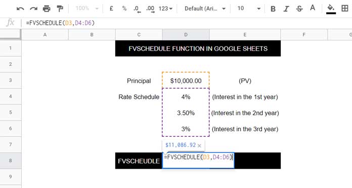
Suppose you invest $10,000 with the following interest rates:

Year 1: 4%
Year 2: 3.5%
Year 3: 3%

Let’s say:

The principal value (PV) is in cell D3.
The rates are in D4:D6.

Your formula in D8 would be:

=FVSCHEDULE(D3, D4:D6)

This will return:

$11,086.92

That’s the future value of your investment after compounding these three varying rates.

FVSCHEDULE function in Google Sheets with example calculation of future value using varying interest rates

Usage Notes

You can specify the rate_schedule in any of these three ways:

1. Percentage Format in Cells

As in the above example, enter values like 4%, 3.5%, and 3% in D4:D6.

2. Using UNARY_PERCENT

This function converts whole numbers into percentage format:

=UNARY_PERCENT(4)    → returns 0.04  
=UNARY_PERCENT(3.5)  → returns 0.035  
=UNARY_PERCENT(3)    → returns 0.03

Place these in cells D4, D5, and D6, respectively.

3. Decimal Format

You can also enter raw decimal values directly into the cells:

0.04, 0.035, 0.03

Or hardcode them directly in the formula:

=FVSCHEDULE(10000, {0.04, 0.035, 0.03})

Important Notes:

Blank cells in the schedule are treated as 0 (i.e., no interest for that period).
If any cell contains text or non-numeric values, the formula will return a #VALUE! error.

Fixed vs. Varying Interest Rates: FVSCHEDULE vs. FV

To understand when to use FVSCHEDULE instead of FV, consider this:

Scenario: Fixed Rate (4% each year for 3 years)

Using FVSCHEDULE (Fixed Rate Example)

=FVSCHEDULE(D3, D4:D6)

If D4:D6 all contain 4%, the formula returns:

$11,248.64

Using FV (Same Fixed Rate)

=FV(4%, 3, 0, -10000)

In this formula:

4% is the annual interest rate
3 is the number of periods
0 is the periodic payment
-10000 represents the initial investment (entered as a negative value)

This formula will return the same result as the FVSCHEDULE example: $11,248.64

When Should You Use FVSCHEDULE?

Use FVSCHEDULE when interest rates vary across periods.
Use FV when the interest rate is fixed throughout.

That’s it! Now you know how to use FVSCHEDULE in Google Sheets to apply multiple interest rates and calculate the future value of your investments.