The N function in Google Sheets returns numbers. When the provided argument is a number, it returns that number; otherwise, it returns 0.
It is not commonly used, as other formulas can replace it to return a number or 0. For example, you can achieve a similar result using =IFERROR(A1*1, 0).
This tutorial explains how to use the N function and provides a real-life example of its use in Google Sheets.
Using the N Function in Google Sheets
We will start with the syntax and basic examples, followed by a real-life example.
Syntax
N(value)In this, value is the argument to be converted. The value is usually a reference to a cell or an array. If you refer to an array or range, you should enter the formula as an array formula. The syntax would be =ArrayFormula(N(range)).
The N function returns 0 in all cases except when the argument is a number, date, time, or Boolean TRUE value.
If the value is:
- A number: returns that number
- TRUE: returns 1
- A date or time: returns a serial number based on the number of days since 30 December 1899
- All other values: return 0
Basic Examples
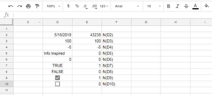
I have entered a few values in the range D2:D10 and used the following formula in cell E2, then dragged it down:
=N(D2)
Starting with the formula in cell E2, the N function converts the date entry in cell D2 to its equivalent date value.
If you check the other formulas, you can see that numbers are returned as the same numbers, the text is converted to the numeric value 0, Boolean TRUE is converted to 1, and FALSE is converted to 0. This behavior (TRUE = 1 and FALSE = 0) also applies to Tick Boxes.
N Function Array Formula Use
As already mentioned, the N function in Google Sheets can also take an array as the argument. For example, you can enter an array formula in cell E2 (please refer to the above screenshot) instead of entering several non-array formulas in the range E2:E10:
=ArrayFormula(N(D2:D10))In some complex formulas involving lookups, you might want to generate #N/A errors in columns instead of an empty string as part of logical tests. In that case, you can use NA().
Example:
=ArrayFormula(IF((A1:A="Apple")+(A1:A="Orange"), "fruits", NA()))This formula converts “Apple” and “Orange” to “fruits” and all other values to #N/A errors.
How to Fill Blank Cells with the Value Zero in a Numeric Field in Google Sheets
In the following screenshot, see the values in the range C1:E4 where the cells D2 and E3 are blank. The following N formula in cell G1 fills those blank cells with 0.
=ArrayFormula(N(C1:E4))
This example is specific to a numeric field. If you apply this to a range that contains mixed data types, it may not be the right choice. Please see the resources section at the bottom.
N Function in MMULT to Avoid #VALUE Error [Practical Use]
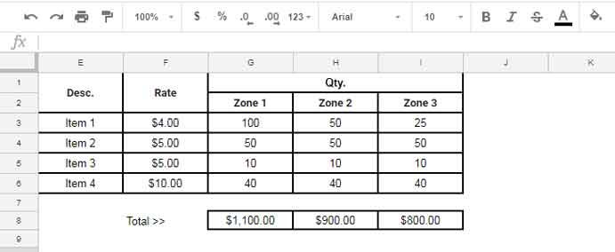
In the following example, we have the rate of items in F3:F6 and quantities from different zones in G3:G6, H3:H6, and I3:I6.
To get the amount below each quantity column, we can use the following MMULT formula in cell G8:
=MMULT(TRANSPOSE(F3:F6), G3:I6)
If you delete any of the values in the range G3:I6 (the quantity columns), MMULT will return a #VALUE error.
We can use the N function to sort this out:
=ArrayFormula(MMULT(TRANSPOSE(F3:F6), N(G3:I6)))When using the N function in a range, be sure to apply ArrayFormula. I hope this makes it clear.


