Free Time Blocking Template in Google Sheets (Smart & Easy to Use)

Time blocking is an advanced version of a to-do list. In a to-do list, you simply enter tasks and check them off once completed. But in time blocking, you assign specific time slots to different activities.

My free smart time blocking template in Google Sheets takes this method further. It lets you pick predefined activities for a day or a whole week, and then gives you a dynamic summary of where you spend your time.

This Google Sheets time blocking template comes with built-in categories, an automated dashboard, and even a doughnut chart that shows exactly how your time is distributed. The layout makes it simple to update your schedule on the go. You don’t need to type anything—just select from drop-down menus once you’ve set it up.

First, we’ll see how to use this time blocking spreadsheet, then we’ll look at one smart formula and the highlight rules that make it powerful. And yes—it’s super easy to set up and use.

Copy the Smart Time Blocking Template (Free)

Table of Contents

How to Use the Free Time Blocking Google Sheets Template

The free weekly time blocking Google Sheets template is made up of three main tabs: Categories, Schedule, and Dashboard.

1. Categories Tab – Set Your Activity Categories

In the Categories tab, replace the existing 12 categories in A2:A13 with your own. Categories are simply the common tasks you want to block time for.

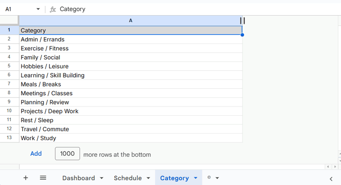
Editable categories in the time blocking planner

I recommend limiting your categories to 8–12:

Too many categories make the system tedious, and you might give up because you spend more time labeling than working.
I’ve created highlight rules for only 12 categories. Beyond that, cells won’t be color-coded.

Keeping categories between 8 and 12 strikes the right balance for an effective smart time blocking planner.

2. Schedule Tab – Plan Your 15-Minute Time Blocks

Now you’re ready to start using the time blocking sheet.

Weekly schedule with 15-minute time slots and selectable tasks

Select the range B4:H99 and delete the dummy data.
Double-click cells in the range to assign your tasks.
Each cell uses a drop-down linked to your categories.

Selecting an activity category in the categories tab

How it works:

The first column lists every 15-minute slot from 00:00 to 23:45.
The next seven columns let you assign categories for each day of the week.

This structure makes it easy to build a daily or weekly time blocking schedule.

Example:

Time	Monday	Tuesday	Wednesday
09:00	Classes / Lectures	Deep Study Block	Meetings
09:15	Classes / Lectures	Deep Study Block	Meetings

3. Dashboard Tab – Track Weekly Summary & Doughnut Chart

The Dashboard tab automatically generates a summary of your week. It shows:

Total time allocated (in hours)
Percentage of total scheduled time
Doughnut chart visualization so you can instantly see time distribution

Example summary:

Dashboard summary showing total hours and doughnut chart of weekly activities

The summary is generated automatically with a formula—no manual work required.

Formulas and Conditional Formatting in the Template

Dashboard Formulas Explained

In cell B2 of the Dashboard tab, I’ve used this formula:

=ArrayFormula(IFERROR(LET(
   ftr, ARRAYFORMULA(
  LET(
    qry, QUERY(TOCOL(Schedule!B4:H99, 1), 
    "SELECT Col1, COUNT(Col1)/4 
     WHERE Col1 IS NOT NULL 
     GROUP BY Col1 
     LABEL Col1 'Activity Category', COUNT(Col1)/4 'Total Time Allocated (Hours)'"),
    col_1, CHOOSECOLS(qry, 1),
    col_2, CHOOSECOLS(qry, 2),
    HSTACK(qry, IFERROR(col_2/SUM(col_2), "Percentage of Scheduled Time"))
  )
), 
   tc, 1, 
   VSTACK(ftr, HSTACK("Total", DSUM(ftr, SEQUENCE(1, COLUMNS(ftr)-tc, tc+1), IFNA(VSTACK(CHOOSEROWS(ftr, 1), )))))
)))

It looks complex, right? But the heart of the formula is this QUERY:

=QUERY(TOCOL(Schedule!B4:H99, 1), 
"SELECT Col1, COUNT(Col1)/4 
 WHERE Col1 IS NOT NULL 
 GROUP BY Col1 
 LABEL Col1 'Activity Category', COUNT(Col1)/4 'Total Time Allocated (Hours)'")

Here’s what it does:

TOCOL flattens the schedule into a single column.
QUERY groups the categories and returns the total time (each count ÷ 4 equals hours, since each slot = 15 minutes).

The remaining part of the formula adds a third column to calculate the Percentage of Scheduled Time and includes a total row. You can read more about this dynamic formula here: How to Calculate Percentage of Grand Total in Google Sheets Query and Dynamic Total Row for FILTER, QUERY, or ARRAY Results in Sheets

👉 For the chart, we don’t need the total row, so I used this formula in cell J2:

=FILTER(CHOOSECOLS(B:D, 1, 3), B:B<>"Total")

and then masked it with background color.

Schedule Tab Automation & Time Slots

The Schedule tab doesn’t really need formulas, but I used this one in cell A4 to create the time slots automatically:

=SEQUENCE(24*4, 1, TIME(0, 0, 0), TIME(0, 15, 0))

This generates time slots at 15-minute intervals from 00:00 to 23:45.

For formatting, I applied 12 highlight rules for each category, plus one additional rule for the hour rows:

=B4=INDIRECT("Category!A2")
=B4=INDIRECT("Category!A3")
...
=B4=INDIRECT("Category!A13")

These rules check each cell and apply colors based on the category selected.

Another rule:

=MINUTE($A4)=0

This highlights the hour rows for better readability.

Why Use This Template?

This free time blocking planner in Google Sheets is:

Free – No hidden costs
Simple – No need for external apps
Customizable – Define your own categories
Detailed – Plan in 15-minute increments
Automated – Dashboard handles calculations for you
Visual – Doughnut chart shows exactly where your time goes

It’s perfect for professionals, students, or anyone who wants to take control of their schedule with a time blocking system.

Final Thoughts

Time blocking is one of the most effective ways to organize your day. With this free time blocking template in Google Sheets, you’ll see exactly how you spend your time—and how to adjust for better balance and productivity.