Formula Auto-updating When Inserting Rows or Columns [Google Sheets]

Let’s first understand what an auto-updating formula in Google Sheets is, and then explore how to meet your specific needs.

You may want your formula to automatically update when you insert or add new rows or columns in Google Sheets. Inserting rows or columns will naturally update the formula.

For example, consider a sheet with 1,000 rows and the following formula in cell B2 that counts the values in the range A2:A1000:

=COUNTA(A2:A1000)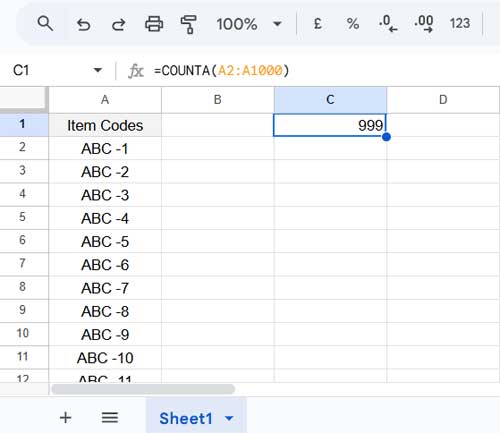

Sample dataset for testing formula auto-updating when inserting rows in Google Sheets

You omit A1 because it contains the column header, which you want to exclude from the count. The formula will naturally count any values inserted between rows 2 and 1,000.

However, when you insert a row between row 1 and row 2, the formula won’t auto-update to include the new row. Similarly, if you add a row after row 1,000, it won’t be included.

We’ve discussed vertical ranges. What about horizontal data?

Let’s assume you have 26 columns in your sheet, from A to Z, and you’re using the following formula to count the values in the range B1:Z1:

=COUNTA(B1:Z1)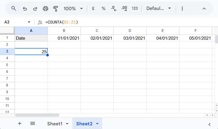

Sample dataset for testing formula auto-updating when inserting columns in Google Sheets

The formula will include the values when you insert any column between B and Z. However, if you insert a column to the left of B or to the right of Z, they won’t be included.

Both COUNTA (for vertical or horizontal ranges) will auto-update but won’t capture the values in newly inserted rows or columns outside the range because of the relative reference nature.

Let’s explore how to include these newly added rows and columns.

Formula Auto-Updating When Inserting Rows in Google Sheets

We will categorize formulas that auto-update when inserting rows under four categories: standard, top open, bottom open, and full open.

Standard (Regular Formula)

This is the regular approach.

Using the example above, the COUNTA formula is as follows:

=COUNTA(A2:A1000)

When you insert one row above A2, the formula will become:

=COUNTA(A3:A1001)

And when you add a row below the 1,000th row, it won’t change.

If you insert one row between row 2 and row 1,000, the formula will become A2:A1001.

That’s the characteristic of the above standard formula.

Top Open (Formula with Open Range at the Top)

The purpose of the formula is to count the values in column A, excluding the header row. The header is in cell A1, so we specified A2:A1000 in the example above. The limitation of this formula is that it won’t capture values when you insert a row between rows 1 and 2, i.e., immediately below the header row. Here’s how to address this:

To capture the rows inserted immediately above the range, replace the formula with the following:

=COUNTA(INDIRECT("A2"):A1000)

When you insert a row above A2, the formula becomes:

=COUNTA(INDIRECT("A2"):A1001)

This will capture the value in the newly inserted row. The logic is that the start range is specified using INDIRECT, so it remains fixed at A2, while the end range (A1000) adjusts automatically.

Aside from this, it behaves like the standard formula when it comes to auto-updating when inserting rows. This means that adding a row after the 1000th row (the last row) has no impact on the formula, but inserting a row between rows 2 and 1000 will include the newly inserted row in the formula.

To fully open the range at the top, replace “A2” with “A1”.

Bottom Open (Formula with Open Range at the Bottom)

To get an open range at the bottom, simply remove the row number from the end part of the reference.

As per our example, you can use:

=COUNTA(A2:A)

The formula will capture any rows added below row 1,000, as per our example.

Full Open (Formula with Open Range at the Top and Bottom)

This depends on your specific requirement. If you want the formula to auto-update when inserting rows anywhere in the sheet, you can use:

=COUNTA(A:A)

This will capture all the rows inserted in the formula.

If you want to freeze the formula at a specific row at the top, for example, row 2, use:

=INDIRECT("A2:A")

Formula Auto-Updating When Inserting Columns in Google Sheets

We’ve seen formulas that auto-update when inserting rows, which is the usual use case. But in cases of horizontal datasets, you might want to apply formulas across the range.

Here are the standard, left open, right open, and full open range references in formulas:

Standard Formula:

=COUNTA(B1:Z1)

This counts the values in B1:Z1. When you insert a column between B and Z, it becomes B1:AA1 and captures the newly inserted column.

Left Open Formula:

=COUNTA(INDIRECT("B1"):Z1)

This will capture any column inserted to the left of column B, i.e., between columns A and B.

To fully open the left range, replace “B1” with “A1”.

Right Open Formula:

=COUNTA(B1:1)

This will include all columns inserted after column Z.

Full Open Formula:

=COUNTA(1:1)

This will include all values in row 1. If you want to freeze the formula at a specific column (e.g., column B), use:

=COUNTA(INDIRECT("B1:1"))

Conclusion

I’ve shared several formulas with clear explanations. Before you start using them, test them in your sheet and ensure you fully understand how they work.

In addition, if you’re using structured tables, you can use structured table references in formulas to auto-update when inserting rows or columns within the table. Please check out my relevant tutorials in the resources below.