The FLIP function lets you dynamically reverse the order of a row, column, or multi-column range in Google Sheets. You can use it with both open and closed ranges.

FLIP is a custom named function in Google Sheets. To use it, you can either import it from my sample sheet or create it within your own sheet. The function will only be available in the specific workbook where it is imported or created.

Before diving into that, let me show you how useful this function is for flipping data in Google Sheets.

FLIP Custom Named Function in Google Sheets: Syntax and Arguments

Syntax:

FLIP(range, direction)  

Arguments:

• range – The data range to flip.
• direction – Specifies the flipping direction:
  • "V" to flip vertically (reverse rows).
  • "H" to flip horizontally (reverse columns).

Example Usage:

Using the FLIP function is simple. Here’s how you can apply it in Google Sheets:

=FLIP(A1:A5, "V")  // Flips column A1:A5 upside down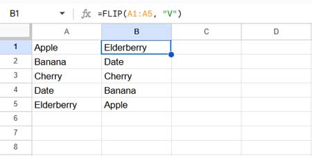

=FLIP(A1:E1, "H")  // Flips row A1:E1 from right to left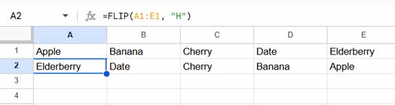

=FLIP(A1:B5, "V")  // Flips all rows in range A1:B5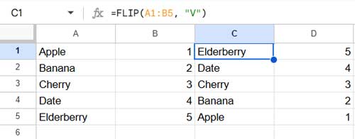

=FLIP(A1:E2, "H") // Flips all columns in range A1:E2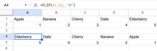

Unlike traditional formulas, you don’t need multiple functions to flip data horizontally or vertically. FLIP handles both in a single formula.

How the Function Handles Empty Rows or Columns

One common challenge when reversing data is dealing with empty rows or columns. Here’s how FLIP handles them:

• If direction is "H", it removes trailing empty columns but keeps empty columns within the range. The function determines the last column with data using the first row of the range.
• If direction is "V", it removes trailing empty rows but retains empty rows within the range. The function identifies the last row with data based on the first column.

This ensures an exact horizontal or vertical flip without unnecessary empty spaces.

Importing the FLIP Custom Named Function

You can import the FLIP function from my sample sheet and use it immediately. If you prefer to create it yourself, skip this section.

Steps to Import:

1. Click the following link to copy my sheet containing the FLIP function.
2. Copy the file name.
3. Open the Google Sheets file where you want to use FLIP.
4. Go to the Data menu and click Named functions.
5. Click Import function in the sidebar panel.
6. Paste the copied file name into the search field.
7. Press Enter to search.
8. Select the copied file and click Insert.
9. A small pop-up will appear with the function code. Select the function and click Import.

You’ll see a message: “Named function imported successfully!”

Now, you can use FLIP across all sheets in that file to reverse data horizontally or vertically.

Creating the FLIP Custom Named Function

If you prefer to create the function yourself, follow these steps:

1. Go to Data > Named functions.
2. Click Add new function in the sidebar panel.
3. Under “Function name”, enter FLIP.
4. Under “Function description”, enter: Reverses the order of rows or columns in the given range. Use "V" for vertical flip or "H" for horizontal flip.
5. Under “Argument placeholders”, enter:
   • range
   • direction
6. Under “Formula Definition”, paste the following formula:

=LET(first, IF(direction="V", CHOOSECOLS(range, 1), IF(direction="H", CHOOSEROWS(range, 1),)), last, ARRAYFORMULA(XMATCH(TRUE, first<>"",0, -1)), IF(direction="H", CHOOSECOLS(range, SEQUENCE(last, 1, last, -1)), IF(direction="V", CHOOSEROWS(range, SEQUENCE(last, 1, last, -1)),)))

7. Click Next.
8. Under “Argument description”, enter:
   • For range: The data range to flip.
   • For direction: Specifies the flipping direction.
9. Under “Argument example”, enter:
   • For range: A1:Z100
   • For direction: "H"
10. Click Create.

Your FLIP function is now ready to use!

Formula Explanation

Even though the formula looks complex, it’s structured logically. I used the LET function to define key variables for reuse:

• first – Extracts the first row or column based on the direction:
  IF(direction="V", CHOOSECOLS(range, 1), IF(direction="H", CHOOSEROWS(range, 1),))
  • If "V", it selects the first column.
  • If "H", it selects the first row.
  • This helps determine the last non-empty cell in the range.
• last – Finds the last non-empty cell in first:
  ARRAYFORMULA(XMATCH(TRUE, first<>"", 0, -1))
• The final step flips the data:
  IF(direction="H", CHOOSECOLS(range, SEQUENCE(last, 1, last, -1)), IF(direction="V", CHOOSEROWS(range, SEQUENCE(last, 1, last, -1)),))
  • If “H”, CHOOSECOLS selects columns from last to first, flipping horizontally.
  • If “V”, CHOOSEROWS selects rows from last to first, flipping vertically.

This efficiently reverses your data while preserving the structure.

Wrap-Up

This tutorial provides an easy-to-use solution for flipping data horizontally or vertically in Google Sheets.

• Import the FLIP() function if you want a quick, ready-to-use solution.
• Create it manually if you want to understand the logic behind it and customize it further.

If you have any questions about the function, feel free to ask in the comments!

Resources

• How to Flip a Column in Google Sheets – Finite and Infinite Columns
• How to Flip a Row in Google Sheets
• Reverse an Array in Google Sheets
• Flip a Table Vertically in Excel (Includes Dynamic Array Formula)