Google Sheets: Create a Dynamic Gantt Chart Timescale

In this post, let’s learn how to create a Dynamic Gantt Chart Timescale in Google Sheets. This setup will help you get adjustable timescale views that respond to different project needs.

Table of Contents

What Does This Do?

Using a drop-down menu, you can switch between different time units—Hours, Days, Weeks, Fortnights, Months, Quarters, Half-Years, and Years. The formula dynamically adjusts your Gantt chart timescale based on the selected unit.

Imagine you want to show Gantt bars across weeks instead of days. You simply pick “Weeks” from the drop-down, and the custom formula will adjust the timeline accordingly.

Flexible Timescale for Gantt Chart in Action

Dynamic Gantt Chart Timescale in action showing adjustable timescale views (GIF)

One note: shorter time units (like Hours or Days) are preferable. With larger units, tasks of shorter durations may not be visible clearly.

Let’s see how to create adjustable timescale views in Google Sheets for your Gantt chart step-by-step.

Step 1: Create a Drop-Down for Time Units

The formula supports the following units:

Hours, Days, Weeks, Fortnights, Months, Quarters, Half-Years, Years

To create the drop-down:

Navigate to cell B1
Go to Insert > Dropdown
Replace Option 1 with “Hours”, Option 2 with “Weeks”, click Add another item, and continue adding all time units.
Click Done

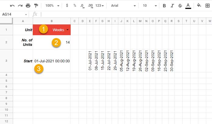
This drop-down in B1 will control the timescale. Our Dynamic Gantt Chart Timescale formula in E3 will generate the timescale units across row E3:3 based on the selection.

Step 2: Enter the Number of Units

Enter the desired number of timescale units in cell B2. This determines the width of your Gantt chart timeline.

For example, enter 14.

Step 3: Enter the Project Start Date

The project start date is essential for generating the Dynamic Gantt Chart Timescale.

Enter the start date in B3. Since “Hours” is one of our units, include the time component too.
For example: 01/07/2021 00:00:00

Drop-down menu for time units and basic input fields for dynamic Gantt chart timescale setup in Google Sheets

Step 4: Formula to Create a Dynamic Gantt Chart Timescale

Clear the range E3:3 and insert the following formula in E3. Then format the range as Date via Format > Number > Date.

=ArrayFormula(
  IF(B1="Hours", TIME(SEQUENCE(1, B2, HOUR(B3), 1), 0, 0),
    IFNA(
      EDATE(B3,
        SEQUENCE(1, B2, 0,
          IFS(B1="Months", 1, B1="Quarters", 3, B1="Half Years", 6, B1="Years", 12)
        )
      ),
      SEQUENCE(1, B2, B3,
        IFS(B1="Fortnights", 14, B1="Weeks", 7, B1="Days", 1)
      )
    )
  )
)

Note:
If the selected unit is “Hours”, change the format to Time via Format > Number > Time.

Formula Explanation

Part 1 – IF (Hours)

Handles the “Hours” unit:

IF(B1="Hours", TIME(SEQUENCE(1, B2, HOUR(B3), 1), 0, 0)

If B1 equals “Hours”, it generates a row of hourly timestamps.

Part 2 – EDATE (Months, Quarters, Half-Years, Years)

EDATE(B3,
  SEQUENCE(1, B2, 0,
    IFS(B1="Months", 1, B1="Quarters", 3, B1="Half Years", 6, B1="Years", 12)
  )
)

This handles date-based jumps using EDATE and is effective for larger intervals.

Part 3 – IFNA (Fallback for Fortnights, Weeks, Days)

SEQUENCE(1, B2, B3,
  IFS(B1="Fortnights", 14, B1="Weeks", 7, B1="Days", 1)
)

Used when the unit doesn’t match any of the EDATE logic—generates incremental days, weeks, or fortnights.

Adjustable Timescale Views in Google Sheets

Once the Dynamic Gantt Chart Timescale in Google Sheets is set, you can now connect it to your task data to visualize progress.

Gantt Bars Based on Dynamic Timescale

Let’s now generate the Gantt bars:

B4: Project End Date (timestamp format)
B5:B10: Task start dates
C5:C10: Task end dates

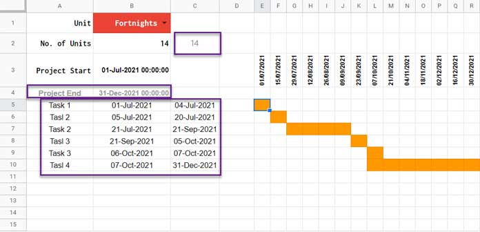
Gantt chart bar visualization based on flexible timescale selection in Google Sheets

Select the range E5:10, then apply Conditional Formatting with the following custom formula:

=AND(E$3 >= $B5, E$3 <= $C5)

This will highlight the cells to represent the Gantt bars based on your selected time unit.

Note:
If using the “Hours” unit, task start/end times in B5:C10 should be in HH:MM:SS format (e.g., 07:00:00).

Optional: Auto-Calculate Number of Units

You can use the formula below in C2 to calculate how many units fall between your project start and end dates (B3 and B4):

=IFS(
  B1="Days", DATEDIF(B3, B4, "d") + 1,
  B1="Months", DATEDIF(B3, B4, "m") + 1,
  B1="Years", DATEDIF(B3, B4, "y") + 2,
  B1="Half Years", ROUNDUP((DATEDIF(B3, B4, "d") + 1) / 182) + 1,
  B1="Quarters", ROUNDUP((DATEDIF(B3, B4, "d") + 1) / 120),
  B1="Fortnights", ROUNDUP((DATEDIF(B3, B4, "d") + 1) / 14),
  B1="Weeks", ROUNDUP((DATEDIF(B3, B4, "d") + 1) / 7),
  B1="Hours", ROUNDUP((B4 - B3) * 24)
)

You can use this in place of manually entering a number in B2.

Conclusion

That’s how you can build a Dynamic Gantt Chart Timescale in Google Sheets with adjustable timescale views using formulas—no add-ons or scripts needed.

Thanks for reading.

Sample Sheet