In this post, you’ll learn how to effectively use the FLATTEN function in Google Sheets to flatten a range. Additionally, I’ll explain how to “unflatten” a previously flattened range using the WRAPROWS function.

Originally, FLATTEN was an undocumented function for quite some time. However, it is now part of the native functions in Google Sheets.

One important thing to note is that you can now use the TOCOL function, which offers additional features beyond FLATTEN. In this post, I’ll also compare FLATTEN with TOCOL, so you can choose the best option for your use case.

Let’s begin with how to use the FLATTEN function in Google Sheets.

FLATTEN Function: Syntax and Arguments

The syntax of the FLATTEN function is:

=FLATTEN(range1, [range2, …])

Arguments:

• range1 – The first range to flatten.
• range2, … – (Optional) Additional ranges to flatten.

Purpose:

The FLATTEN function takes the input ranges and flattens them into a single column by scanning row-by-row. It processes the first row, then the second, and so on.

Examples of the FLATTEN Function and Comparison with TOCOL

In the example below, the array A1:D is flattened into rows in F1:F.

=FLATTEN(A1:D)

Screenshot #1:

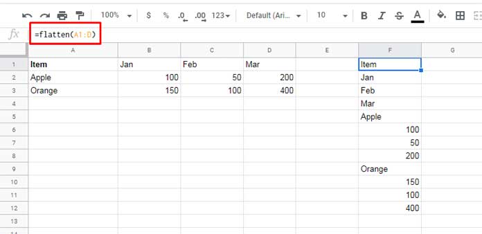
The equivalent TOCOL formula for this is:

=TOCOL(A1:D)

The advantage of using TOCOL here is that it allows you to remove empty cells and errors from the flattened data. To do this, you can use the formula:

=TOCOL(A1:D, 3)

This makes TOCOL more versatile for many situations.

If you want to flatten specific ranges individually, like in the formula below:

=FLATTEN(A1:A3, B1:B3, C1:C3, D1:D3)

Screenshot #2:

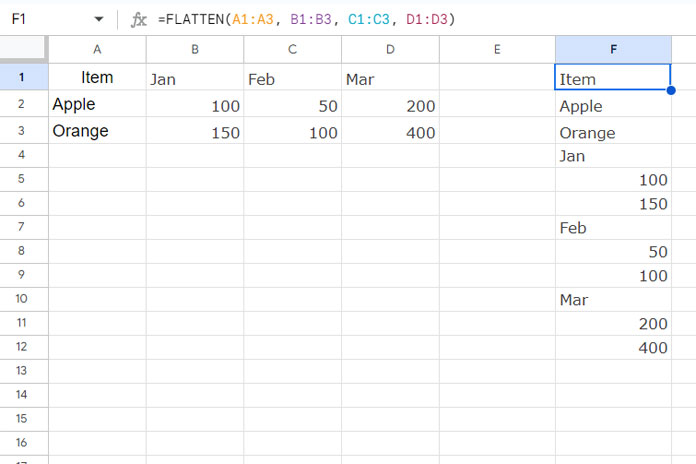
Each range will be stacked one after another in the output. The TOCOL equivalent would be:

=TOCOL(A1:D3, ,TRUE)

This version of TOCOL flattens the array by column instead of row.

Real-Life Use Case: Unique Scattered Values and Summary

You can use the FLATTEN function in various real-life scenarios in Google Sheets. Here’s an example where we use FLATTEN to gather unique or summarize scattered values in a sheet.

For instance, consider the berth preferences of passengers. To find the unique preferences and a summary:

The usual UNIQUE formula, like this:

=UNIQUE(B2:D)

won’t give the desired result because it works across columns. Instead, you can use:

=UNIQUE(FLATTEN(B2:D))

This formula in cell F2 will provide the unique values from the scattered data.

Screenshot #3:

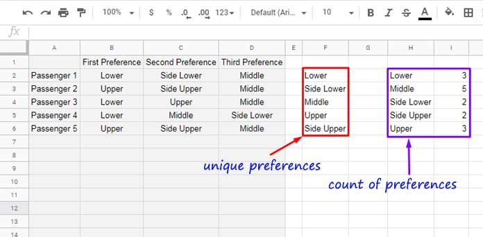
To generate a summary of these preferences, use the following QUERY formula in cell H2:

=QUERY(FLATTEN(B2:D), "SELECT Col1, COUNT(Col1) WHERE Col1 IS NOT NULL GROUP BY Col1 LABEL COUNT(Col1) ''")

This query will count the occurrences of each unique value in the flattened data.

How to Unflatten a Flattened Range in Google Sheets

To “unflatten” a previously flattened range, you can use the WRAPROWS function.

Referring to Screenshot #1, let’s take the flattened values in the range F1:F. To unflatten this data, we need to determine how many values should be placed in each row.

Based on the original dataset in A1:D, we know the range contains 4 columns, meaning each row contains 4 values.

Therefore, we can use the WRAPROWS function with a wrap count of 4 to unflatten the data. Here’s the formula in H1:

=WRAPROWS(F1:F12, 4)

This formula will restore the flattened data back into its original 4-column format.

Resources

• A Simple Formula to Unpivot a Dataset in Google Sheets (Using FLATTEN)
• How to Move Each Set of Rows to Columns in Google Sheets
• How to Partially Flatten a Multi-Column Array in Google Sheets
• How to Flatten Every Other Column in Google Sheets