If you’re building reports or dashboards in Google Sheets, you may often need to focus only on the most recent business days, excluding weekends. This is especially useful when you’re tracking performance, generating summaries, or analyzing trends over active business days.

With an array formula, you can dynamically calculate and display the last 7 business days based on today’s date—no manual updates needed.

Use Cases for the Last 7 Working Days:

• Filtering tables to show only recent workday activity
• Tracking daily sales or expenses over the most recent business week
• Generating team productivity or task completion reports
• Creating rolling dashboards for KPIs that exclude weekends
• Preparing automated client or internal reports without weekend data

Formula to Find the Last 7 Business Days in a Column

Sample Data:

Example showing the last 7 working days (highlighted).

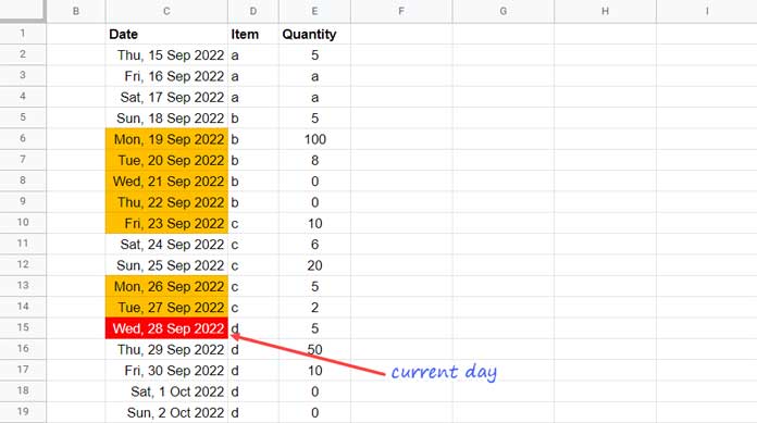
As per the screenshot example, the current day is 28/09/2022. That’s the value Google Sheets returns if you use =TODAY() in any cell.

The cells highlighted in amber represent the last 7 business days.

In cell F2, enter the following formula and drag it down as needed:

=AND(WORKDAY(C2 - 1, 1) = C2, ISBETWEEN(C2, WORKDAY(TODAY(), -7), TODAY() - 1))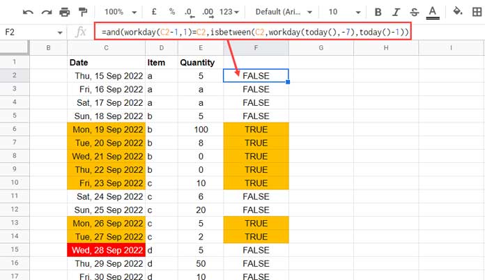

Finding the Last Seven Business Days (Formula Logic)

Let’s break down the logic:

You want to test whether each date in column C:

1. Falls within the range of the last 7 business days (excluding today)
2. Is itself a valid business day

Condition 1:

=WORKDAY(C2 - 1, 1) = C2

This checks whether the date in C2 is a valid business day.

Condition 2:

=ISBETWEEN(C2, WORKDAY(TODAY(), -7), TODAY() - 1)

This checks whether the date falls within the last 7 business days before today.

Combine both conditions using:

=AND(condition_1, condition_2)

Array Formula to Get the Last 7 Business Days in Google Sheets

If you prefer a formula that spills down automatically and marks the last 7 business days, use this array formula:

=ArrayFormula((WORKDAY(C2:C - 1, 1) = C2:C) * ISBETWEEN(C2:C, WORKDAY(TODAY(), -7), TODAY() - 1))

Enter it in cell F2 after clearing any existing formulas in column F.

The logic is the same as above. Since AND() doesn’t work in arrays, we use the multiplication operator * to combine conditions.

Note: This formula returns TRUE (1) or FALSE (0) for each row. TRUE (1) marks the last 7 business days.

Number the Last 7 Business Days from Today (1 to 7)

If you’d rather return numbers 1 to 7 (starting from today and counting backward), use this formula:

=ArrayFormula(IFNA(XMATCH(C2:C, ArrayFormula(WORKDAY(TODAY(), SEQUENCE(7, 1, -1, -1))))))

This generates the last 7 business days and matches each date in column C to its corresponding rank.

How to Exclude Specific Weekends and Holidays

By default, the above formulas treat Saturday and Sunday as weekends. If you need custom weekends (e.g., only Sunday), use the WORKDAY.INTL function:

WORKDAY.INTL(start_date, num_days, [weekend], [holidays])

Refer to the Google Sheets documentation for weekend number options.

Related Resources

• Filter the Last N Days of Data in Google Sheets
• Same Day Last Week Comparison in Google Sheets
• Finding the First and Last Workdays of a Month in Google Sheets
• Get Last 7, 30, and 60 Days Total in Each Row (from Today) in Google Sheets
• Find the Last Saturday of Any Month in Google Sheets (Easy Formula)
• How to Find the Last Working Day of a Year in Google Sheets
• How to Find the Last Business Day of a Month in Excel
• Filter the Last 7 Days in Excel Using the FILTER Function