The best way to find duplicates in new lines inside cells in Google Sheets is to use conditional formatting.

This post explains how to highlight duplicates in the second line inside cells in a column and across rows.

We will use a custom formula (highlight rule) to achieve this since there is no built-in rule within the Conditional formatting dialog panel.

There are two examples below: The first one is the column example, and the second one is the across-the-row example.

So there will be two rules but similar in characteristics.

Before beginning, if you do not know how to add new lines, please don’t forget to check the “Resources” at the end of this post.

Here we go!

How Do We Find Duplicates in New Lines Inside Cells in a Column?

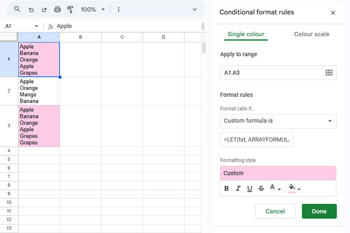
You can use the built-in conditional formatting feature to highlight duplicates in new lines inside cells in a column in Google Sheets.

Here are the steps to follow:

The following steps are for the range A1:A.

Please modify it to find/highlight duplicates within cells in a different range.

1. Select the cell range you want to check for duplicates in new lines.
2. Go to the “Format” menu, then choose “Conditional formatting.”
3. In the “Format cells if” dropdown menu (immediately under the “Format rules”), select “Custom formula is.”
4. In the “Value or formula” field, enter the formula given immediately after the seventh step below.
5. Replace A1 and $A$1:$A1 with the first cell in your selected range.
6. Choose the formatting style you want to apply to the duplicates in new lines in the selected cell range.
7. Click “Done” to apply the formatting.

Formula Rule (Column):

=ArrayFormula(not(regexmatch(trim(regexextract(A1&"","\n.*")),"^"&textjoin("$|^",1,unique(trim(ifna(regexextract($A$1:$A1&"","\n.*"))),false,true))&"$")))

It will highlight cells in column A wherever duplicate values appear in new lines within each cell.

Anatomy of the Rule: Extracting Second Line Values in Cells and Analyzing

We can peel the above rule and see how each part help to highlight duplicates in new lines inside cells in A1:A in Google Sheets.

Part _1

The first thing to do is extract the value in the second line from cell A1.

Using REGEXEXTRACT, we can extract any characters after the linefeed (newline) character.

We should trim the result to remove any additional white space characters.

=trim(regexextract(A1&"","\n.*"))

Please note we have used A1, the first cell in the range and relatively referenced.

So it will automatically become A2, A3, A4, and so on in the selected cells down in Conditional formatting.

Part_2

Here is a similar formula for $A$1:$A1, with additional modifications.

=ArrayFormula(unique(trim(ifna(regexextract($A$1:$A1&"","\n.*"))),false,true))

Note:- In the rule that highlights duplicates in new lines, you will only see the above-bolded part. Nesting of ARRAYFORMULA is not necessary for most of the Google Sheets formulas.

The cell range in the above formula part becomes $A$1:$A2, $A$1:$A3, $A$1:$A4, in the cells down.

The first cell is absolute, and the second cell is relative.

Here are the other changes compared to part_1.

The IFNA removes #N/A errors, and UNIQUE gets distinct values (values that do not repeat).

The purpose of part two is to create a regular expression. So removing the #N/A error is necessary.

Part _2_a

The TEXTJOIN combines the extracted part_2 values and forms a regular expression.

=ArrayFormula("^"&textjoin("$|^",1,unique(trim(ifna(regexextract($A$1:$A1&"","\n.*"))),false,true))&"$")

We are ready to highlight duplicates in new lines inside cells in a column.

Part_3

Let’s conclude the steps.

Our final REGEXMATCH formula that finds duplicates in new lines in a column is as follows.

=ArrayFormula(not(regexmatch(part_1,part_2_a)))

Part_1: The new line value in the current row.

Part_2_a: The distinct values in new lines up to the current row.

Logic:- Part_1 doesn’t match part_2_a means it already appears in the range in new lines. So duplicate.

That’s the logic behind finding duplicates in new lines in a column in Google Sheets.

How Do We Find Duplicates in New Lines Inside Cells Across Rows?

How do we apply the above formula in a table?

The above formula won’t support highlighting duplicates in new lines across rows.

We require to modify the regular expression part, which is part_2_a.

This time we have a few records in the range A1:D10, which means in multiple rows and columns.

We want to highlight new line duplicates row-wise. Here is that formula rule.

Formula Rule (Across the Row):

=ArrayFormula(not(regexmatch(trim(regexextract(A1,"\n.*")),"^"&textjoin("$|^",1,unique(trim(ifna(regexextract($A1:$D1,"\n.*"))),true,true))&"$")))

Select A1:D10 and apply it as instructed earlier.

One of the changes in comparison to example # 1, i.e., Formula Rule (Column), is within UNIQUE.

Syntax:

UNIQUE(range, [by_column], [exactly_once])

Earlier, the data was in a single column. So we followed the below syntax to get the distinct values.

UNIQUE(range, false, true)

Now it’s across the row. So here is the syntax in use.

UNIQUE(range, true, true)

Resources

• Start New Lines Within a Cell in Google Sheets – Desktop and Mobile.
• How to Move New Lines in a Cell to Columns in Google Sheets.
• Remove Whitespaces at the Beginning of a Newline in Google Sheets.
• Extract Every Nth Line from Multi-Line Cells in Google Sheets.