I couldn’t find any built-in option to filter the top 10 items in the Google Sheets Pivot table. You may require a custom formula for that.

In Excel, I could see a top 10 filter option under the ‘Value filters’ in Pivot table reports.

Using that feature in Excel, we can filter top ‘n’ values in the Pivot table. That Excel feature helps us to filter the bottom 10 values too.

Let’s hope that Sheets’ development team will include such a feature in the Google Sheets Pivot table sooner or later.

See the Excel Pivot table filter option first.

Google Sheets Pivot table lacks these Value Filters by Top 10 or Bottom 10 (to see Bottom 10, you should first click Top 10 in Excel). 

Instead, in Google Sheets, you can use custom formulas for this type of filtering presently.

The Pivot table editor in Google Sheets has a conditional filter option.

In this post, you can learn how to code a custom formula to filter by bottom/top 10, or you can say bottom/top ‘n’ items in the Pivot table in Google Sheets.

Filtering Top 10 Items by Values in Pivot Table in Google Sheets

The Pivot table contains aggregated data. In that, we are going to apply the filter. But there is one key point to note!

Write a custom formula based on the source range (A1:B), not on the pivot range (E1:F) (please see the screenshot below for the range reference).

That doesn’t mean you can’t use a custom formula in the Pivot Table based on the pivot range. But in our case, I mean to filter the top 10 values in the Pivot table, use the source range A1:B.

From my testing, the Pivot range E1:F won’t work correctly in custom formulas.

The Formula Logic Behind Filtering Top 10 Pivot Table Items in Google Sheets

Since we use a custom formula to filter the top 10 Pivot table items based on their values, we must know how to group and aggregate the source data.

We can use SUMIF or Query for this. I will use the Query function to extract the top 10 item names (not quantity) based on their aggregated (grouped) quantities.

First, we will filter the top 3 Pivot table items by their values. We can later easily convert these top 3 values to the top 10.

The top 3 items by their values (Qty) are “Product 1”, “Product 6”, and “Product 10” (later we will learn how to find them).

We can use the following formula to filter these values in the custom formula field in the Pivot table editor > Filters > Add > Product > Filter by condition > Custom formula.

=regexmatch(Product,"^Product 1$|^Product 6$|^Product 10$")

In this Regexmatch formula, the Product is the field label (column name).

The other part of the formula, i.e., "^Product 1$|^Product 6$|^Product 10$", is the top 3 items separated by pipe symbols.

The caret and dollar signs match the start and end of a line, respectively. It avoids partial matches of texts (products).

We can use the Regexmatch formula in Google Sheets to match multiple texts in an array.

See the syntax of this Google Sheets text function.

REGEXMATCH(text, regular_expression)

Please go through the above formula and this syntax.

You can understand that the filed label containing the product names is the text argument, and the top 3 items separated by pipe is the regular_expression (here, the text to match).

Custom Formula to Filter a Pivot Table Items by Top 10 Values

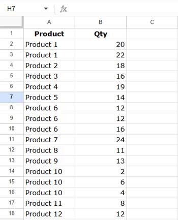
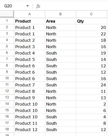
Let’s start creating a Pivot table first. I have slightly modified the values in columns A and B. You can see those changes in the below image.

Pivot Table – Single Column

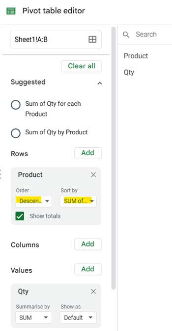
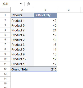
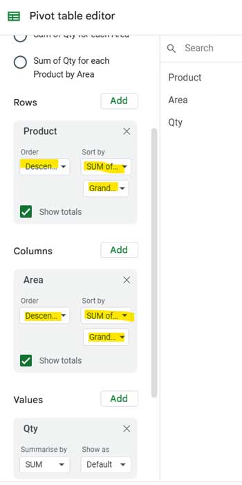
In this report, I have grouped the ‘Product’ in ‘Rows’ and added ‘Qty’ to the Values field to Sum.

In addition to that, I sorted ‘Product’ in the Pivot table in descending order based on the ‘SUM of Qty.’

From this, you can quickly identify (not filter) the top 10 products. Now the custom filter formula part.

Pivot Table and Query Formula – Side by Side

We can replicate the above Pivot table using a Query formula, and here it is.

=query({A1:B18},"Select Col1,Sum(Col2) group by Col1 order by Sum(Col2) desc")

From this, we want to extract the top 10 items. For that, include the Limit clause in Query, which limits the number of rows returned.

=query({A1:B18},"Select Col1,Sum(Col2) group by Col1 order by Sum(Col2) desc limit 10")

You May Like: Learn Google Sheets Query Function: Step-by-Step Guide.

Now we can form a regular expression to match these top 10 items.

Regular Expression to Match Top 10 Items in Google Sheets Pivot Table

The above Query returns two-column data. We only want the first column that contains the item names. Also, we don’t want the header.

You can remove the header by omitting row # 1 in the Query data. For that, use the data range {A2:B18} instead of {A1:B18} in Query.

Also, remove the second column field label ‘sum Qty’ (see the cell I1 on the above image) by adding the Label clause, label Sum(Col2)'', in Query.

Then to remove the second column, use another Query wrapping the first one.

=query(query({A2:B18},"Select Col1,Sum(Col2) group by Col1 order by Sum(Col2) desc limit 10 label Sum(Col2)''"),"Select Col1")

Now we are set to form the regular expression.

Join the above string output with the pipe, caret, and dollar signs as below.

^Product 1$|^Product 6$|^Product 7$|^Product 4$|^Product 2$|^Product 3$|^Product 5$|^Product 9$|^Product 10$|^Product 12$

How do we do that?

We can do it in two steps.

1. Use & (ampersand) to add the caret sign as the prefix and the dollar sign as the suffix to each value.

=ArrayFormula("^"&query(query({A2:B18},"Select Col1,Sum(Col2) group by Col1 order by Sum(Col2) desc limit 10 label Sum(Col2)''"),"Select Col1")&"$")

I have wrapped the formula with the ArrayFormula function since we used the ampersand in an array of values.

2. Finally, use Textjoin to insert the pipe.

=ArrayFormula(textjoin("|",1,"^"&query(query({A2:B18},"Select Col1,Sum(Col2) group by Col1 order by Sum(Col2) desc limit 10 label Sum(Col2)''"),"Select Col1")&"$"))

Regexmatch Formula to Filter Top 10 Items in Google Sheets Pivot Table

As I have mentioned in the beginning, use the above regular expression in the Regexmatch.

Formula # 1:

=regexmatch(Product,ArrayFormula(textjoin("|",1,"^"&query(query({A2:B18},"Select Col1,Sum(Col2) group by Col1 order by Sum(Col2) desc limit 10 label Sum(Col2)''"),"Select Col1")&"$")))

It’s for use within the Pivot table editor, not in a cell.

Applying Custom Formula in Google Sheets Pivot table

We now have the formula to filter the Pivot table in Google Sheets by the top 10 items.

Steps to Add a Custom Formula in Google Sheets Pivot table:

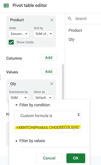
1. Click the ‘Add’ button against ‘Filters’ on the Pivot table editor.
2. Choose the field ‘Product’ from the drop-down as we want to match the product names.
3. On the drop-down menu that appears, you will see the default filter set to ‘Showing all items.’ Click that and choose Filter by condition > Custom formula.
4. Copy and Paste the above formula in the blank field there, click the OK button, and voila!
5. If you want to filter the top 5 items in the Pivot table, change the number 10 in the Query Limit clause to 5.

How to Filter Bottom 10 Items in Google Sheets Pivot Table

Once you have learned the above custom filter, you can easily tweak the formula to filter the bottom 10 or bottom ‘n’ items in the Google Sheets Pivot table.

Change the sort order in the Query from desc to asc. That is the only change required to filter the bottom 10 items in the Pivot table in Google Sheets.

Formula # 2:

=regexmatch(Product,ArrayFormula(textjoin("|",1,"^"&query(query({A2:B18},"Select Col1,Sum(Col2) group by Col1 order by Sum(Col2) asc limit 10 label Sum(Col2)''"),"Select Col1")&"$")))

Also, if you want, change the sort order in the Pivot table editor panel. Just sort the ‘Product’ field under the ‘ROWS’ to any order.

Top or Bottom N Items in Multiple Column Pivot Table in Google Sheets

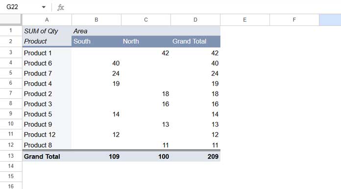
In the above Pivot table examples, we have only one category field, i.e., Product. What about one more field or a subcategory called ‘Area’?

In that case, include that additional column in the Query Select and Group by clause as below.

Previous Query with One Category (Top 10):

=query({A2:B18},"Select Col1,Sum(Col2) group by Col1 order by Sum(Col2) desc limit 10 label Sum(Col2)''")

Query with Two Categories (Top 10):

=query({A2:C18},"Select Col1,Col2,Sum(Col3) group by Col1,Col2 order by Sum(Col3) desc limit 10 label Sum(Col3)''")

The outer Query and other elements (the Textjoin and Regexmatch) will be the same.

The below formula filters the top 3 items in a multi-column Pivot table in Google Sheets.

Formula # 3:

=regexmatch(A2:A18,ArrayFormula(textjoin("|",1,"^"&query(query({A2:C18},"Select Col1,Col2,Sum(Col3) group by Col1,Col2 order by Sum(Col3) desc limit 3 label Sum(Col3)''"),"Select Col1")&"$")))

To filter the bottom 3 items, needless to say, change the sort order in the Limit clause in Query.

Formula # 4:

=regexmatch(A2:A18,ArrayFormula(textjoin("|",1,"^"&query(query({A2:C18},"Select Col1,Col2,Sum(Col3) group by Col1,Col2 order by Sum(Col3) asc limit 3 label Sum(Col3)''"),"Select Col1")&"$")))

Additional Customization – Include Duplicates in the Top N Values

You might see one difference when you compare my custom formula-based Pivot table filtering output with the Excel built-in top 10 filterings.

The Excel Pivot table doesn’t filter out duplicates, but my custom formulas do that. Let’s go deep into that.

Single Column Pivot Table

Let’s start with Formula # 1, which filters the top 10 items in the Pivot table.

Change that formula to filter the top 4 values as below.

=regexmatch(Product,ArrayFormula(textjoin("|",1,"^"&query(query({A2:B18},"Select Col1,Sum(Col2) group by Col1 order by Sum(Col2) desc limit 4 label Sum(Col2)''"),"Select Col1")&"$")))

As you can see, I have only changed Limit 10 to 4.

Then change the value in cell B4 to 19. We require to do that to generate a duplicate in top #4.

You will get a different output in Excel and Google Sheets. Here is that result comparison.

Excel	Sheets
Product 1 – 42	Product 1 – 42
Product 6 – 40	Product 6 – 40
Product 7 – 24	Product 7 – 24
Product 2 – 19	Product 2 – 19
Product 4 – 19

You can see that Excel returns one additional (fifth) row, and the ‘SUM of Qty’ is equal to the fourth row ‘SUM of Qty.’

If you want Excel similar output, I mean top n values with duplicates in the Pivot table, make the below changes in your Formula # 1 above.

Change this Query part of the formula;

query({A2:B18},"Select Col1,Sum(Col2) group by Col1 order by Sum(Col2) desc limit 4 label Sum(Col2)''")

to;

sortn(query({A2:B18},"Select Col1,Sum(Col2) group by Col1 label Sum(Col2)''"),4,3,2,0)

We removed the Order By and Limit clauses in Query. The SORTN takes care of that, and it also helps to retain the duplicates.

When using SORTN with Query, use the second argument of it to control N. Here, the number 4 is the second argument in SORTN and which represents ‘n’ items.

What about Formula # 2, i.e., bottom ten values?

First, change that formula to filter the top 3 values as below by replacing Limit 10 to Limit 3.

Here is that Query part (without duplicates).

query({A2:B18},"Select Col1,Sum(Col2) group by Col1 order by Sum(Col2) asc limit 3 label Sum(Col2)''")

Modify it to (with duplicates);

sortn(query({A2:B18},"Select Col1,Sum(Col2) group by Col1 label Sum(Col2)''"),3,3,2,1)

Multiple Column Pivot Table

I have used my custom Formula # 3 (scroll to the top to see) to filter top n values in a multi-column Pivot table. I have used Formula # 4 to filter bottom n values.

To include duplicates, you can use SORTN with Query as below.

Note:- You will see different numbers in the Limit clauses in the original Query formulas above (Formulas 3 and 4). I’m modifying that below so that you can see duplicates.

Formula # 3 earlier Query (without duplicates);

query({A2:C18},"Select Col1,Col2,Sum(Col3) group by Col1,Col2 order by Sum(Col3) desc limit 4 label Sum(Col3)''")

to be replaced with (with duplicates);

sortn(query({A2:C18},"Select Col1,Col2,Sum(Col3) group by Col1,Col2 label Sum(Col3)''"),4,3,3,0)

Formula # 4 earlier Query (without duplicates);

query({A2:C18},"Select Col1,Col2,Sum(Col3) group by Col1,Col2 order by Sum(Col3) asc limit 3 label Sum(Col3)''")

to be replaced with (with duplicates);

sortn(query({A2:C18},"Select Col1,Col2,Sum(Col3) group by Col1,Col2 label Sum(Col3)''"),3,3,3,1)

One more thing. When you use open ranges such as A2:C in Query, don’t forget to filter out duplicates by using the Where clause.

E.g.:

sortn(query({A2:C18},"Select Col1,Col2,Sum(Col3) Where Col1 is no null group by Col1,Col2 label Sum(Col3)''"),3,3,3,1)

Pivot Tables Examples