In many scenarios, you may want to filter rows in a range where all columns contain text in Google Sheets. For example, in a customer feedback table, you might expect all the columns to be filled with relevant information. Leaving empty cells in any column or inserting random numbers may not be sufficient to qualify the feedback.

To filter rows where all columns have text, we will use a combination of functions, with FILTER playing a key role.

Generic Formula

Here is the formula to filter rows where all columns contain text content in Google Sheets:

=FILTER(range, MMULT(--ISTEXT(range), SEQUENCE(COLUMNS(range), 1, 1, 0)) = COLUMNS(range))

In this generic formula, replace range with the specific range you want to filter.

Example: Filter Rows Where All Columns Contain User Feedback in Text

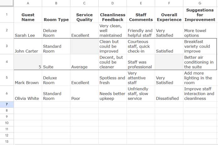
In the following example, a hotel feedback table collects user experiences. Some users may fail to enter names and may instead input random numbers to hide their identities. Additionally, they might skip providing important feedback.

We want to filter the rows where all columns are filled with text content.

The range in our example is A1:G. Here’s the formula to filter rows in the range A1:G where all columns contain text content:

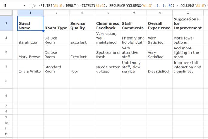
=FILTER(A1:G, MMULT(--ISTEXT(A1:G), SEQUENCE(COLUMNS(A1:G), 1, 1, 0)) = COLUMNS(A1:G))

Formula Breakdown

To understand this formula, it’s important to break down and explain the condition that filters the rows.

The formula syntax is:

FILTER(range, condition1, [condition2, ...])

Where:

• range = A1:G (the range to filter)
• condition1 = MMULT(--ISTEXT(A1:G), SEQUENCE(COLUMNS(A1:G), 1, 1, 0)) = COLUMNS(A1:G)

Let me explain the condition1 in detail so you can understand how the formula filters rows where all columns contain text.

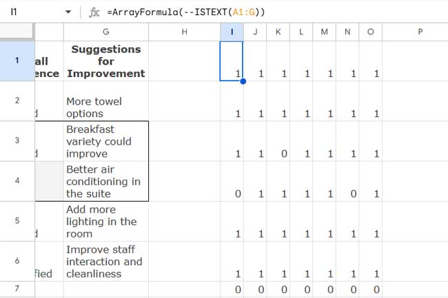
1. --ISTEXT(A1:G): This part converts the result of the ISTEXT function (which checks if a cell contains text) into a numeric array. It returns 1 for text values and 0 for non-text (or empty) cells. The -- (double negation) converts the TRUE/FALSE result into 1/0.
   
2. SEQUENCE(COLUMNS(A1:G), 1, 1, 0): This generates a vertical array of numbers starting from 1, with a length matching the number of columns in the specified range (in this case, A1:G). The SEQUENCE function creates a sequential array that helps in multiplying with the results from ISTEXT to check each column.
   {1; 1; 1; 1; 1; 1; 1}
3. MMULT(--ISTEXT(A1:G), SEQUENCE(COLUMNS(A1:G), 1, 1, 0)): The MMULT function performs matrix multiplication between the array of text (converted to 1/0) and the sequence of numbers. This gives the sum of the 1s (representing text values) across each row. If all columns in a row contain text, the sum will equal the total number of columns in that row.
4. = COLUMNS(A1:G): This checks if the sum from the MMULT function matches the total number of columns in the range (i.e. if the sum of 1s equals the total number of columns). If it does, it returns TRUE, meaning all columns have text content. If not, it returns FALSE.
5. FILTER(range, condition): The FILTER function returns the rows where the condition evaluates to TRUE, i.e., where all columns contain text.

The formula will return all rows where every column contains text content. Rows with empty or non-text values in any of their columns will be excluded.

Resources

• Formula to Filter Uppercase | Lowercase | Proper Case Text in Google Sheets
• Filter Out If the Entire Row Is Blank in Google Sheets