


")


")

")
")
 in Excel & Google Sheets")


This tutorial walks you through filtering multiple columns in Google Sheets using both the Filter menu and the FILTER function, enabling you to refine your data efficiently.
The Filter menu lets you apply filters directly to the source data, allowing you to view and modify the filtered content as needed.
The FILTER function extracts matching data into a separate range, helping you focus on specific conditions while keeping the original dataset unchanged.
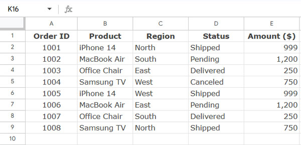
Sample Data
Our sample dataset contains five columns: Order ID, Product, Region, Status, and Amount. We will apply filters to columns C (Region) and D (Status).
Filtering Multiple Columns with Multiple Conditions
We will apply two types of filters to refine the data:
- AND Condition: Displays only the rows where the Region is “North” and the Status is “Shipped.”
- OR Condition: Displays rows where the Region is “North” or the Status is “Shipped.”
Filter Multiple Columns Using the Filter Menu
You can filter one column at a time using the Filter menu, but to filter multiple columns, you need to use a custom formula. When writing the formula, avoid selecting the entire range; using just the first data row (the row below the header) is sufficient.
Steps:
1. Click on cell C1 (or any column header where you want to apply the filter).
2. Go to Data > Create a filter.
3. Click the drop-down arrow in cell C1 to open the Filter menu.
4. Select Filter by condition and choose Custom formula is.
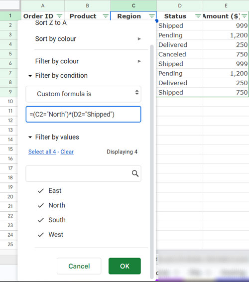
5. Enter one of the following formulas:
AND Condition:
=(C2="North")*(D2="Shipped") // Filters rows where Region is "North" AND Status is "Shipped"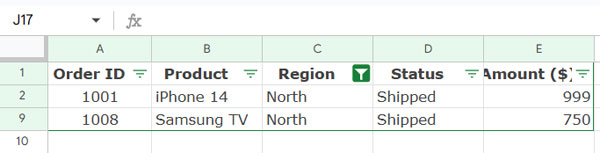
OR Condition:
=(C2="North")+(D2="Shipped") // Filters rows where Region is "North" OR Status is "Shipped"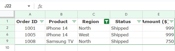
6. Click OK to apply the filter.
This method allows you to filter multiple columns in Google Sheets directly within the source data.
Filter Multiple Columns Using the FILTER Function
If you want to extract the filtered data into a new range instead of modifying the original dataset, use the FILTER function.
Formula 1: AND Condition
=FILTER(A2:E, (C2:C="North")*(D2:D="Shipped"))(Filters rows where Region is “North” AND Status is “Shipped”)
Formula 2: OR Condition
=FILTER(A2:E, (C2:C="North")+(D2:D="Shipped"))(Filters rows where Region is “North” OR Status is “Shipped”)
The FILTER function dynamically updates your filtered data when you add new entries.
Pros and Cons of Filtering Methods
Here’s a quick overview of the advantages and disadvantages of using the Filter menu and the FILTER function for filtering multiple columns of data.
| Method | Pros | Cons |
| Filter Menu | Directly filters the source data | Doesn’t auto-update when new data is added |
| FILTER Function | Creates a separate filtered dataset that updates dynamically | Cannot edit the filtered data directly |
If you need an interactive filter, the Filter menu is useful. If you need dynamic filtering, the FILTER function is the better choice.
Resources
- Multi-Condition Filtering in the Same Column (Google Sheets)
- Create a Drop-Down for Filtering Rows and Columns
- Filtering When Columns Contain Merged Cells in Google Sheets
- Select All or a Specific Category in Multiple Columns in Filter in Google Sheets
- Filter Data Using a Multi-Select Drop-Down in Google Sheets
- Filter Rows Containing Multiple Selected Values in Google Sheets