")
")


")


")

")
")
 in Excel & Google Sheets")


Google Sheets now allows selecting multiple values in drop-downs, making it easier to filter data dynamically. However, there’s a challenge—selected values are stored as comma-separated text, making filtering difficult with standard formulas.
This tutorial explains how to filter data using a multi-select drop-down in Google Sheets. That means you will filter a column based on multiple criteria selected in a drop-down menu using an efficient formula.
Challenges in Filtering Multi-Select Drop-Down Data
The issue with filtering multi-select drop-down data is that the selected criteria appear as drop-down chips, but in reality, they are stored as comma-separated values. To use them as criteria in the FILTER function, we need a different approach.
Formula to Filter Data Using a Multi-Select Drop-Down
Use the following generic formula:
=FILTER(range, XMATCH(criteria_range, SPLIT(criteria, ", ", FALSE)))Where:
range– The range of data to filter.criteria_range– The column to evaluate.criteria– The cell containing the multi-select drop-down.
Example: Filtering Data Using a Multi-Select Drop-Down
Let’s consider the following sample data in A1:B, where column A contains items and column B contains their colors:
| Item | Color |
|---|---|
| Shirt | Black |
| Jacket | Red |
| Pants | Blue |
| Shoes | Green |
| Scarf | Black |
| Hat | Grey |
| Gloves | Brown |
| T-shirt | Yellow |
| Sweater | Teal |
You want to filter the items by colors, such as all items in black color or all items in black or red color. To achieve this:
Step 1: Create a Multi-Select Drop-Down
- Navigate to cell D1.
- Click Insert > Drop-down.
- In the sidebar, select ‘Drop-down (from a range)’.
- Click the ‘Select data range’ icon and enter
B2:Bin the pop-up. - Click OK, then check “Allow multiple selections”.
- Click Done.
Now, cell D1 contains a multi-select drop-down based on the unique values in column B.
Step 2: Apply the FILTER Formula
Enter the following formula in cell E2:
=FILTER(A2:B, XMATCH(B2:B, SPLIT(D1, ", ", FALSE)))How This Formula Works:
SPLIT(D1, ", ", FALSE)– Splits the multi-select drop-down values into an array.XMATCH(B2:B, ...)– Matches each value in column B against the split array.FILTER(A2:B, ...)– Filters rows where a match is found.
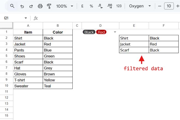
Expected Output:
If you select Black, Red in cell D1, the filtered result will be:
| Item | Color |
| Shirt | Black |
| Jacket | Red |
| Scarf | Black |
Key Takeaways
- Multi-select drop-downs store values as comma-separated text.
- The SPLIT function helps convert them into an array for filtering.
- The XMATCH function efficiently finds matches.