")


")


")

")
")
 in Excel & Google Sheets")


The FACT function in Google Sheets is a handy tool under the Math category. It calculates the factorial of a non-negative number, which is essential when working with permutations and combinatorics.
In mathematics, factorial (denoted by n!) represents the product of a whole number and all the positive integers less than it. It’s used to determine the number of ways to arrange a set of distinct objects.
For example, the letters X, Y, and Z can be arranged in 6 different ways:
XYZ, XZY, YXZ, YZX, ZXY, ZYXThat’s because:
3! = 3 × 2 × 1 = 6Let’s see how to use the FACT function in Google Sheets to compute factorials like this.
FACT Function in Google Sheets – Syntax and Arguments
FACT(value)value – A non-negative number or cell reference for which you want to calculate the factorial.
Notes
- If
valueis not an integer, it is truncated (e.g., 3.9 becomes 3). - If the referenced cell is blank, Google Sheets treats it as 0, and
FACT(0)returns 1. - If the input is text, the result is
#VALUE!. - If the value is negative,
FACTreturns#NUM!.
Formula Examples
Example 1 – Using a Hardcoded Number
=FACT(3)Returns 6.
Example 2 – Using a Cell Reference
If B2 contains the number 3, use:
=FACT(B2)Returns 6.
Array Formula Usage of the FACT Function in Google Sheets
Want to calculate the factorials of numbers 1 to 10? Here are three different ways:
Method 1 – Manual Fill (Non-Array Formula)
- Enter numbers 1 to 10 in cells A1:A10
- In B1, enter:
=FACT(A1) - Copy down to B10
Method 2 – Apply FACT to a Range with ArrayFormula
=ArrayFormula(FACT(A1:A10))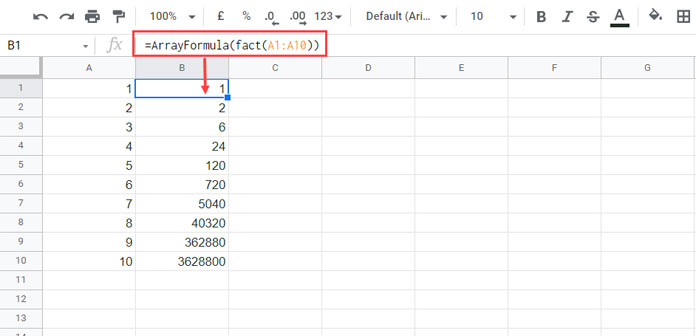
Put this in B1 to compute all 10 factorials at once.
Method 3 – Use SEQUENCE to Generate Numbers
=ArrayFormula(FACT(SEQUENCE(10, 1)))No need to manually input numbers. SEQUENCE(10, 1) generates values from 1 to 10.
Inverse Factorial in Google Sheets
What if you’re given a factorial value like 3628800, and you want to find the original number? In other words, you want to compute the inverse factorial in Google Sheets.
Here’s a formula that does just that:
Formula to Get Inverse Factorial in Google Sheets
Assume A1 contains the factorial value.
=XMATCH(1, SCAN(A1, SEQUENCE(1000), LAMBDA(acc, val, acc/val)))How the Inverse Factorial Formula Works
SEQUENCE(1000)generates numbers from 1 to 1000.- SCAN starts with the factorial value in cell
A1and keeps dividing it by each value in the sequence. - The LAMBDA defines how each step divides the accumulated result by the next number in the sequence. The
accparameter holds the intermediate result at each step. - When the result becomes exactly
1, we know we’ve reversed all the factorial multiplications. XMATCH(1, …)returns the position where the result equals 1 — that is, the original number whose factorial is inA1.
Tip – Adjust Range If Needed
If the formula returns #N/A, increase 1000 to a higher number to search a larger range.
Conclusion
The FACT function in Google Sheets makes it easy to calculate factorials for everything from simple math problems to advanced permutations.
And with a little creativity, you can even compute the inverse factorial in Google Sheets, making your spreadsheet truly dynamic.
Thanks for reading!