


")


")

")
")
 in Excel & Google Sheets")


When using the QUERY function in Google Sheets, combining conditions with AND, OR, and NOT is essential for filtering data effectively. However, without using parentheses to define precedence, the function may return unexpected results.
This guide explains how to use these logical operators correctly—including how to explicitly define precedence for accurate results.
Sample Sheet: Click here to copy the sample sheet. Use this sheet to explore and test each example covered in the sections below.
This tutorial is part of the WHERE Clause in Google Sheets QUERY: Logical Conditions Explained hub, which covers all logical operators, comparisons, and condition-building patterns used in QUERY statements.
1. Introduction to Logical Operators in QUERY
In Google Sheets QUERY, the WHERE clause is used to filter rows based on conditions. Logical operators—AND, OR, and NOT—allow you to combine multiple conditions.
These logical operators let you create complex filtering logic, such as:
- This AND that
- This OR that
- NOT this
- A combination of
ANDandOR
But to ensure your logic is evaluated correctly, you must use parentheses when combining AND and OR.
2. Basic Syntax of AND, OR, and NOT
OR: Match Any Condition
=QUERY(A1:E7, "SELECT * WHERE B='First' OR B='Second'", 1)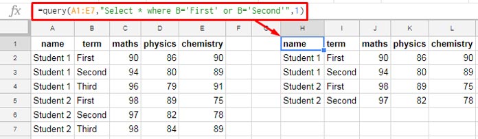
Returns rows where column B is either “First” or “Second”.
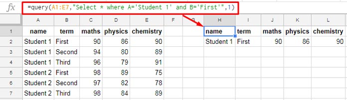
AND: Match All Conditions
=QUERY(A1:E7, "SELECT * WHERE A='Student 1' AND B='First'", 1)Returns rows where column A is “Student 1” and column B is “First”.
NOT: Exclude a Condition
=QUERY(A1:E7, "SELECT * WHERE A='Student 1' AND NOT B='First'", 1)Returns rows where column A is “Student 1” but column B is not “First”.
Result:
| name | term | maths | physics | chemistry |
| Student 1 | Second | 94 | 80 | 89 |
| Student 1 | Third | 96 | 79 | 91 |
You can also use:
B != 'First'
B <> 'First'
as alternatives to NOT.
3. Why Parentheses Matter (Explicit Precedence)
When combining AND and OR, Google Sheets QUERY does not automatically follow traditional logical precedence. You must use parentheses to ensure the correct order of evaluation.
Let’s look at two formulas using the same student dataset in A1:E7.
❌ Incorrect Formula (No Parentheses):
=QUERY(A1:E7, "SELECT A WHERE C>95 OR D>95 AND B='First'", 1)This is evaluated as:
- C > 95
- OR (D > 95 AND B = “First”)
As a result, students with C > 95 will be included even if B ≠ “First”—which may not be what you want.
✅ Correct Formula (With Parentheses):
=QUERY(A1:E7, "SELECT A WHERE (C>95 OR D>95) AND B='First'", 1)This ensures the condition evaluates correctly:
- (C > 95 OR D > 95)
- AND B = “First”
Only students who scored more than 95 in either C or D and also have “First” in column B will be returned.
4. Common Examples
OR in the Same Column
=QUERY(A1:E7, "SELECT * WHERE B='First' OR B='Second'", 1)OR Across Different Columns
=QUERY(A1:E7, "SELECT A WHERE C>95 OR D>95 OR E>95", 1)Find students scoring more than 95 in any subject.
AND in Different Columns
=QUERY(A1:E7, "SELECT * WHERE A='Student 1' AND B='First'", 1)Combined AND + OR (With Precedence)
=QUERY(A1:E7, "SELECT * WHERE A='Student 1' AND (B='First' OR B='Second')", 1)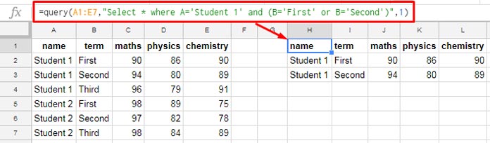
NOT with Null Check
=QUERY(A1:E, "SELECT * WHERE A IS NOT NULL", 1)5. What Happens Without Parentheses?
Without parentheses, QUERY may evaluate your conditions in an unexpected order.
For instance, a formula like:
=QUERY(A1:E7, "SELECT A WHERE C>95 OR D>95 AND B='First'", 1)will treat it as:
- C > 95
- OR (D > 95 AND B = “First”)
This means students with only C > 95 will still appear—even if they don’t belong to the “First” group. To fix this, wrap the OR part in parentheses:
=QUERY(A1:E7, "SELECT A WHERE (C>95 OR D>95) AND B='First'", 1)6. Tips and Best Practices
- Always use parentheses when combining
ANDandOR. - Use
<>or!=as alternatives toNOT, especially for text and numeric comparisons. - For checking empty values, use
IS NOT NULL. - Use comments or notes in your sheet to document complex queries.
That’s all about using AND, OR, and NOT in Google Sheets QUERY—with an emphasis on defining explicit precedence. Try using these tips in your formulas and enjoy more accurate, powerful filtering!
Thank you!! Solved it!! Good explanation 🙂
Hi Prashanth,
I am having trouble to generate the expected result using “is not null” function.
=QUERY('Sheet1'!$A$1:$F$81; "select * where E is not null"; 1)The column E contains dates, but in somes cases, text, as I want to show two or more dates.
Example:
Column E
2/3/23
2/4/22
18/5/21
2/9/22 ; 11/6/21
I only get the results from rows with a proper date.
I hope you can help me to show all the cells that are not empty.
Thank you.
Hi, Federico,
That’s what happens with a mixed data column. The minority data types, text values in your case, are considered null values.
So use the FILTER() instead.
=filter(Sheet1!A1:F81;len(Sheet1!E1:E81))If you want, you can wrap this result with QUERY for further aggregation.
Hi Prashanth,
I am having trouble trying to generate the expected result using query.
Here is the scenario, the columns are:
Column A = Features
Column B = Date
Column C = Status (either Option1 or Option2)
My objective is to display all Features having either Option1 or Option2 as their Status given a specific Date (i.e. 3/27/2023).
This is what I have so far:
=query(A2:C, "Select A,C WHERE B = '3/27/2023' AND (C contains 'Option1' OR C contains 'Option2')",0)This is the error I am getting:
Error
Query completed with an empty output.
Hope you can help me out on this.
Thank you.
Hi, Raymond,
You are using the date criterion in the wrong syntax.
Try this.
=query(A2:C, "Select A,C WHERE B = date '2023-03-27' AND (C contains 'Option1' OR C contains 'Option2')",0)Hello,
Excellent post!
I’m having trouble querying data from a column that doesn’t match two other columns.
I have a list of regulars in A. In B, a list of guests.
I combine those 2 in C with
=filter({$A$2:A;$B$2:$B}; LEN({$A$2:A;$B$2:$B})First Team A is the odds
=query($C$2:$C; "SELECT * skipping 2 limit 7";0)and the first Team B is the evens from C=query(query($C$2:$C; "SELECT * OFFSET 1";0);"select * skipping 2 limit 7";0)Now, the next team should be made up of the next 7 from the list.
I can’t find a way to query C where C doesn’t match or is different from G and H.
Can anyone help?
Hi, Ramon Fonseca,
Here are the formulas for the first two teams.
Formula 1 (Team 1)
=query(filter(C2:C,iseven(row(C2:C))),"Select * limit 7 offset 0")Formula 2 (Team 2)
=query(filter(C2:C,isodd(row(C2:C))),"Select * limit 7 offset 0")To get the next two teams (3 and 4), replace
offset 0withoffset 7in both formulas.In the third and fourth formulas, it must be 14.
Oh my – great! Thank you!
I have spent today surely half of the day exploring your tutorials and surely improving my knowledge, but I’m stuck on something again for a few hours: – URL removed by admin –
Thank you again.
Hi, Dech,
I’ve found two issues.
1. You are wrongly specifying dates in the Query. Please check How to Use Date Criteria in Query.
2. Want to get all data when criteria are empty. Please check The Purpose of WHERE 1=1 in Google Sheets Query.
I’ve added a solution in J34.
Hi Prashanth, could you please look at my simple sample sheet?
Since I’m new to the Query function, still after reading many of your articles, I’m not able to do, very likely, a simple task – I need to filter out some data out of the Query result.
The condition is that SUMs <0 should be filtered out.
Here is a simple example: —removed by admin—
Hi, Dech,
Just wrap your query formula with one more query to filter out the values from the sum column.
I’ve already entered the formula in your sheet.
I added a new pivot table too. You can learn pivot table filtering from an example here – How to Filter Top 10 Items in Google Sheets Pivot Table.
Oh my …, the formula in the pivot table is insane 🙂 I would rather stay with the query for now 🙂
Thank you!
Hi Prashanth, I need your help with this formula. Please suggest where I am missing. It works fine without numeric values as criteria.
Column formats:
Col11 = Text
Col2 = Text
Col5 = Numeric
Col6 = Numeric
=QUERY(IMPORTRANGE('EFE Emp Code!A:O'),"Select Col2,Col3,Col4,Col7,Col8,Col9,Col11,Col12,Col13,
Col14 where Col11='"&A2&"' or Col2='"&B2&"' or Col5=
"&C2&" Col6="&D2&"")
Hi, Amit Jain,
You are missing one logical operator OR in the last part. It should be
Col5="&C2&" or Col6="&D2&"").Hi Prashant,
Thanks for your support.
Still, it’s not working! Getting the error “Unable to parse query string for Function QUERY parameter 2: PARSE_ERROR: …”
Please suggest.
Thanks & Regards,
Amit Jain
Hi, Amit Jain,
To solve the Query in person, I require access to your sheet or a copy.
If willing, share it (URL) with editable rights in your reply below. I won’t publish that comment.
I want to filter my data using dates and additional texts with the dates.
I came up with this, but it only filters by date and not with the additional text input.
— Formula Removed —
Hi, Ishan Shah,
Your formula was not helpful to understand the issue.
Make a sample sheet and feel free to share its URL in the reply below.
Hi, Prashanth! I thought I followed your tutorial to the letter, but I’m still getting a “query completed with an empty output” error.
Below is a link to the sheet. Can you help? The formula is in cell I5. Thanks so much!
Here’s a link to the sheet: — removed by admin —
Hi, Julianna,
You have mixed-type data in column D (text and dates). That may cause issues in QUERY.
This FILTER will work.
=filter($B$8:$F$114,datevalue($D$8:$D$114)<=$L$2)If you are particular to use QUERY, you can first use FILTER to filter dates in column D, then use QUERY.
=query(filter($B$8:$F$114,datevalue($D$8:$D$114)),"Select * where Col3<= date '"&TEXT($L$2,"yyyy-mm-dd")&"'",0)Hello,
I have a list of training participants and created a list of drop-downs to help narrow down the query.
Dropdowns:
C2 – Training
C3 – Trainer
C4 – District
C5 – Training Participant ID #
Formula:
=QUERY({'2021-2022'!A1:1000}, "SELECT * WHERE Col1='"&$C$2&"' AND Col8='"&$C$3&"' AND Col7='"&$C$4&"' AND Col2='"&$C$5&"'")How to return a value if one or two of the drop-downs are left blank?
Hoping you can help.
Thank you!
Hi, Briana,
I hope I can help you learn it.
Enter the below formulas in three cells.
Part of Your Exiting Formula:
="SELECT * WHERE Col1='"&$C$2&"' AND Col8='"&$C$3&"' AND Col7='"&$C$4&"' AND Col2='"&$C$5&"'"Modifed 1:
="SELECT * WHERE "&if(C2="","","Col1='"&$C$2&"' AND ")&"Col8='"&$C$3&"' AND Col7='"&$C$4&"' AND Col2='"&$C$5&"'"Modified 2:
="SELECT * WHERE "&if(C2="","","Col1='"&$C$2&"' AND ")&if(C3="","","Col8='"&$C$3&"' AND ")&"Col7='"&$C$4&"' AND Col2='"&$C$5&"'"Delete the criteria in cell C2, then C3. Check what the three formulas return.
Hi Prashanth, could you please help me out with the formula below?
=iferror(Transpose(query(A:B,"Select A where A contains '"&index(split(B4," "),1,1)&"' or A contains '"&index(split(B4," "),1,2)&"'",-1))," ")I’m trying to compare all substrings within a cell with all substrings within another cell.
It isn’t working, but I’m not sure why.
Thank you for your help!
Hi, Camila,
It seems you can solve that using a Regex-based formula, not a Query.
E.g.:-
=regexmatch(A1,regexreplace(B1," ","|"))I can try if you share a sample Sheet below.
Your work is really good, and your explanations are excellent! I was wondering if there is an Ebook version or if you have anything else coming out? Thank you for what you do – you help so many people!
Hi, Karen Brown,
I withdrew my ebooks last year. I think it was a wise decision because it was not selling as expected. Being a non-native English speaker, I have my drawbacks 🙂
Thank you for this post! This is excellent information, and the links back to other posts are very helpful for a better understanding.
My question is – is there a limit to the number of OR statements you can use? I have a query where I’m attempting to bring back vacation (col H), personal (Col I), sick (Col J), and bereavement (Col K) where there is a value of ‘1’ marked in the dataset.
The query brings back all the vacation and personal time throughout the range, but it does not bring back any sick or bereavement records.
My query:
=query('TimeTrack'!E5:K,"Select E,H,I,J,K where H = '1' OR I = '1' OR J = 1 OR K = 1",1)There are values for both Sick (Col J) and Bereavement (Col K) – but no data pulls back. Can you see what is wrong?
Thank you so much!
Hi, Karen Brown,
There are issues with your formula. But to correct that, you must first check the values in the columns H to K.
If column H contains numbers, it should be specified in the formula
H = 1. If it’s text, it should be specified asH = '1'. It applies to other columns also.Oh no! I see my formula is inconsistent with the values! Yes, they are all text, and once I fixed the single quotes around the H and K values – it all works fine. This is an awesome formula!!! Thank you so very much!
Hi Prashanth,
hope you can help me.
Looking for a query alternative of this formula.
=filter(Data!A2:AS,((Data!L2:L =List!B2)*(Data!E2:E >= List!C2))+
((Data!L2:L =List!B3)*(Data!E2:E >= List!C3))+
((Data!L2:L =List!B4)*(Data!E2:E >= List!C4))+
((Data!L2:L =List!B5)*(Data!E2:E >= List!C5)
This formula goes on and on. Tried using query myself using AND and OR but no luck. List contains Employee number and Date. Any suggestions?
Hi, Micole,
I don’t think you require to use QUERY for this. I do have a solution using FILTER itself. Let me explain it below.
IMPORTANT! I am only considering the range Data!A2:L.
Steps:
1. Insert the following formula in Data!M2.
=ArrayFormula(ifna(vlookup(L2:L16,List!B2:C,2,0)))2. Here is the alternative to your FILTER.
=filter(Data!A2:A,regexmatch(Data!L2:L,"^"&textjoin("$|^",true,List!B2:B)&"$")*(Data!E2:E >= Data!M2:M))
I’ll explain it with an example in my next tutorial.
Hello Prashanth,
Another great article. Really helpful stuff. Thank you for sharing.
I do have a question. I am querying based on multiple cell values with the OR operator. All cell values are numeric. Here is my formula:
=iferror(Query('Main Tracking Sheet'!$C$7:$BU,"Select C,D,E,G,H,I,K,O,Q,BT,BN,BS Where BH="&D2&" or BH="&E2&" or BH="&F2&" Order by BT Desc Limit "&H2&"",0))The problem I am having is that if all three cells (D2, E2 & F2) have values, then the query works correctly listing data that match all three conditions.
However, if any one of them is blank, a ‘value’ error results. No matter what I do I cannot get it to work with a blank cell.
I could do really long nested if formulas to check for blank cells, with different formulas for each case …… but that seems like a really ugly solution. To quote the master, Code (complex formulas) must have good taste!
Would deeply appreciate any insight.
Hi, Sharat Goswami,
You can try the below Query.
=iferror(Query('Main Tracking Sheet'!$C$2:$BU,"Select C,D,E,G,H,I,K,O,Q,BT,BN,BS Where BH matches "&"'"&textjoin("|",true,D2:F2)&"'"&"Order by BT Desc Limit "&H2&"",0))For the formula explanation, please follow the below guide.
How to Use Multiple OR in Google Sheets Query.
Brilliant! That worked right out of the gate.
You also helped me figure out how to set up a dynamic hyperlink using the result of a Vlookup.
That was a little piece of genius really! Although in my case I adapted it to use
Cell("row" ....instead of a double substitute. But the basic idea of appending this to regular link to the sheet was quite brilliant, I thought. And those are not the only things I picked up from here. Indirect is another neat one.I mention this so that you know that your work here is indeed helping people who need it.
So thanks Prashanth.
Hi, Sharat,
Thanks for your valuable feedback!
Leaving here the link of the post that you were talking about – Create Hyperlink to Vlookup Output Cell in Google Sheets.
Keep visiting…
Hi Prashanth,
I hope you can assist here!
Column range H:J is where my data are and I need to return the data if what I type in Column G matches column H — what is the best way to go about this?
Hi, Cassie,
Assume your data is in Sheet1. In Sheet2 (which should be blank), in cell A1, insert the below FILTER formula.
=filter(Sheet1!H1:J,Sheet1!G1:G=Sheet1!H1:H)Hello,
I’m hoping you can help! I’m trying to run a query on a range of cells and I’m not sure where I went wrong.
=QUERY('Form responses 1'!A2:BO, "SELECT C, D, E, F, G, H, I WHERE I='Arabic' or WHERE J:BO='Arabic'")I need it to return the data if the choice ‘Arabic’ is in column I or columns J through BO. Any suggestions?
Thanks!
Hi, Alex,
This Query may help.
=QUERY({'Form responses 1'!A1:BO,transpose(query(transpose('Form responses 1'!I1:BO),,9^9))}, "SELECT Col3, Col4, Col5, Col6, Col7, Col8, Col9 WHERE Col68 contains 'Arabic'",1)Hi all,
Please help! I want to QUERY data from a range based on two conditions:
If A=B4 and the date is between two dates (in cells). My formula is:
=query(Database!$A$1:$L,"select B, C, D, F, G, H, I where A='"$B$4"'and (G >= date '"&text($B$2,"yyyy-mm-dd")&"' and G <=
date '"&text($B$3,"yyyy-mm-dd")&"')", 1)
But it gives me an #ERROR! Formula Parse error.
Thank you for your help!
Hi, Matteo,
You were very close!
Just replace
'"$B$4"'with'"&$B$4&"'in your Query formula.Thank you so much! It worked! What does the
'&'do in this case?Hi, Matteo,
As per the syntax
QUERY(data, query, [headers]), thequeryis entered as a text. I mean it’s within double-quotes. So to make a cell reference to work you should enter it like that.Thank you so much. Very helpful and clear.
Hi all,
I am struggling with this formula:
QUERY(Data!B:T,"Select B,G,K,O where T="C2" and N="C3" and Q="F2" and S="F3" and P="I2" Order By G Desc Limit 5")It is throwing a parse error. Can anyone help?
Hi, Kate Greenaway,
I guess the cells C2, C3, F2, F3, and I2 contains the criteria. Since you have not specified whether the criteria are string, number, or dates I am unable to give you the formula. Because each criterion specified differently in the Query.
This tutorial may guide you in the right direction.
Examples to the Use of Literals in Query in Google Sheets.
I want to run a query using WHERE and I want the query to extract data based on two criteria both in the same column.
This is my formula.
query(Dump!J3:V,"SELECT K,L,P,Q,U,V * WHERE Q = '87-Tire Shop' and Q= '487-Tire Sales'",0)I only want those specific columns of data, and only the ones that meet the two different criteria in Col. Q. What is the error?
Hi, mark Denomme,
Remove the asterisk in the SELECT clause and use the OR operator instead of AND operator in the WHERE clause.
=query(Dump!J3:V,"SELECT K,L,P,Q,U,V WHERE Q = '87-Tire Shop' or Q= '487-Tire Sales'",0)You can also use MATCHES instead of OR.
=query(Dump!J3:V,"SELECT K,L,P,Q,U,V WHERE Q matches '87-Tire Shop|487-Tire Sales'",0)Separate each criterion with a pipe.
Search “Complex String Comparison Operators in Query” within this post to get the link to the concerned tutorial.
Self taught google coder looking for help on this formula:
=IFERROR(ARRAYFORMULA(QUERY('NEED APPOINTMENT'!$A$3:$AQ,"Select * Where AH = 15 and AN, AX, BB, BF, BJ, BN is null ")), )Hi, David Salmonsen,
The Query ‘data’ in your formula doesn’t contain the columns AX, BB, BF, BJ, and BN. Further, you should use the AND operator individually with columns. I don’t find the logic in using the ArrayFormula.
In my opinion, the formula should be as below.
=QUERY('NEED APPOINTMENT'!$A$3:$BN,"Select * Where AH = 15 and AN='' and AX='' and BB='' and BF='' and BJ='' and BN =''")You can rewrite the same in this way too.
=QUERY({'NEED APPOINTMENT'!$A$3:$BN},"Select * Where Col34 = 15 and Col40='' and Col50 ='' and Col54 ='' and Col58 = '' and Col62 ='' and Col66 =''")I need help to correct my formula.
I am trying to put conditions to calculate the results.
=query(A8:AG,"Select A,J,U,D,G,I where x= "SW",count(Z) group by A,J,U,D,G,I",1)Hi, Hiten,
The Query clause order is not correct. It should be as below.
=query(A8:AG,"Select A,J,U,D,G,I,count(Z) where X='SW' group by A,J,U,D,G,I",1)Hi Prashanth!
Great article! I’m having some trouble using the NOT function in my formula, could you review and let me know what I’m doing wrong?
=QUERY(IMPORTRANGE("URL","Data!A1:n"),"Select Col1,Col3,Col4,Col7,Col8,Col9,Col10,Col13 Where Col4<20 and Col13'My Text'")
The above formula works until I hit the “and” and “not”. I want to filter out any instances of “My Text” but still, keep rows in Column 13 that have no text/text other than “My Text”.
Hi, Megan,
This may help you.
=QUERY(IMPORTRANGE("Your_URL_Here","Data!A1:N"),"Select Col1,Col3,Col4,Col7,Col8,Col9,Col10,Col13 Where Col4<20 and not Col13='My Text' and not Col13=''")Hi, please help. I need a combination of AND and OR in Query too. I’m having errors here. It keeps duplicating the entries on my data.
I would like the following to get all rows where:
1. Col12 is not ‘Money’
2. Col13 is not ‘Salary’ or not ‘x’
3. Col14 does not contain the words ‘FGD’, ‘Conclave’ or ‘Townhall’
=QUERY (A:Z, "select * where not Col12 contains 'Money' and not Col13 contains 'Salary' and Col13'x' and not Col14 contains lower('FGD') and not Col14 contains lower('Conclave') and not Col14 contains lower('Townhall')")Please note that these are just samples, not real data.
Hi, Leeshean,
Conditions 1 and 2 can be easily written using the AND Query logical operator. But for the third condition, that is multiple doesn’t contain, we can use the MATCH string comparison instead of the CONTAINS string comparison.
Here is the required formula. You may check your sheets Locale settings if you encounter a parse error.
If the data A1:Z is not within curly braces or an expression (output of other functions), then the column identifiers must be A, B, N, etc. instead of Col1, Col2, Col14.
Regarding the multiple contains and not contains using MATCH, to learn the usage, see this post.
Multiple CONTAINS in WHERE Clause in Google Sheets Query
Hi Prashanth,
I need your help. I want to Query from a table that needs to combine both AND and OR operators.
The condition is that there are two types of columns which are DATE and NOTE. I need to ‘Query’ all of the dates in a certain range, where the NOTE column is null.
If there is anything in the NOTE column, I do not want it. This is my formula,
Dates: L, N, P, R, T
Notes: M, O, Q, S, U
=QUERY(OVERALL!A2:Z, "Select B, C, E, F, H, I, J, K, L, M, N, O, P, Q, R, S, T, U, V, W, X, Y, Z where (L >=date '" & AC3 &"' and L =date '" & AC3 &"' and N =date '" & AC3 &"' and P =date '" & AC3 &"' and R =date '" & AC3 &"' and T <=date '" & AC4 &"' and U is null)")This formula works but it only checked the first Date & Notes column which is L & M and if M is not null, it will stop checking.
I need to Query the other columns even if the ones at the front are not null.
Hi, Manisahhh,
For me, the formula seems doesn’t match your explanation.
“…it only checked the first Date & Notes column which is L & M…”.
I could not find the use of column M in your formula.
I don’t know why you are using L greater than or equal (GTE) to the date in cell AC3 and again L equal to the date in cell AC3?
Do you want to omit all the rows containing notes in any column or all the columns?