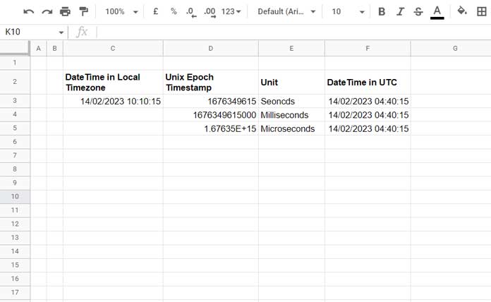
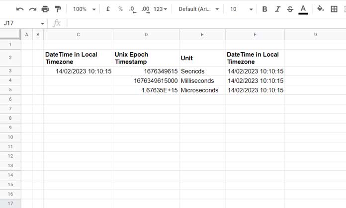
When you have a Unix epoch timestamp in seconds, milliseconds, or microseconds, you can convert that to a DateTime using the EPOCHTODATE function in Google Sheets.

The converted DateTime (timestamp) will be in UTC. But, you can get the local time by adding a timezone offset.

Most of you are probably here to learn the function for future use.

If that is the case, you may not have a Unix epoch timestamp (also known as Unix time, POSIX time, or Unix timestamp) for testing.

So what we will do here is first convert a given DateTime to Unix epoch timestamps in seconds, milliseconds, and microseconds.

Then use the EPOCHTODATE function to convert them back to our local DateTime. That will be quite interesting, right?

Let’s understand the function and arguments first.

Syntax and Arguments

Syntax of the EPOCHTODATE Function in Google Sheets:

EPOCHTODATE(timestamp, [unit])

Arguments:

Timestamp:- A Unix epoch timestamp.

Unit:- The unit of time (in seconds, milliseconds, or microseconds) in which the timestamp is expressed.

You can leave the unit or input 1 for seconds, 2 for milliseconds, or 3 for microseconds.

How to Use the EPOCHTODATE Function in Google Sheets

As mentioned at the beginning of this tutorial, we would first convert a local timestamp to Unix epoch timestamps.

Then we will use the EPOCHTODATE function to convert them. Here are those steps.

Prerequisites

I have the timestamp (DateTime) 14/02/2023 10:10:15 in the format dd/mm/yyyy hh:mm:ss in cell C3.

Please note that the Unix Time is the seconds since 1st Jan 1970 (Epoch). So, use a date greater than 01/01/1970 for testing.

Also, my timezone (IST) is ahead of GMT by 5:30 Hours. So I’ve used -time(5,30,0) in the formulas below.

You must adjust this parameter based on your GMT offset (use the - operator if it is ahead and the + operator if it is behind).

Here are related two tutorials:

• How to Convert a Timestamp to Milliseconds in Google Sheets.
• Convert Unix Timestamp to Local DateTime and Vice Versa in Google Sheets.

The following formulas in cells D3, D4, and D5 convert the value in C3 to Unix epoch timestamps.

D3 (Unix Epoch Timestamp in Seconds):

=(C3-DATE(1970,1,1)-time(5,30,0))*86400

D4 (Unix Epoch Timestamp in Milliseconds):

=(C3-DATE(1970,1,1)-time(5,30,0))*86400000

D5 (Unix Epoch Timestamp in Microseconds):

=(C3-DATE(1970,1,1)-time(5,30,0))*86400000000

Let’s convert these Unix epoch timestamps to DateTime in UTC using the EPOCHTODATE function in Google Sheets first.

EPOCHTODATE Function to Convert DateTime to UTC

We already have the Unix epoch timestamps in seconds, milliseconds, and microseconds in cell range D3:D5.

In F3:F5, we will use the EPOCHTODATE function to convert them into Universal Time Coordinated (UTC).

F3 Formula:

=EPOCHTODATE(D3,1)

F4 Formula:

=EPOCHTODATE(D4,2)

F5 Formula:

=EPOCHTODATE(D5,3)

EPOCHTODATE Function to Convert DateTime to Local Time

As you can see in the above examples, the results do not match the value in C3.

The reason is the EPOCHTODATE function returns the dates in UTC, and the C3 value is in the local timezone.

If you want the converted date in your local timezone, you may ± your GMT offset from the returned date.

In my case (my timezone is ahead of GMT by 5:30 Hours), it will be like this:

F3:

=EPOCHTODATE(D3,1)+time(5,30,0)

F4:

=EPOCHTODATE(D4,2)+time(5,30,0)

F5:

=EPOCHTODATE(D5,3)+time(5,30,0)

That’s all about how to use the EPOCHTODATE function in Google Sheets.